In addition to mathematical expectation and dispersion, probability theory also uses a number of numerical characteristics that reflect certain features of the distribution.
Definition. Fashion Mo(X) random variable X is its most likely value(for which the probability r g or probability density
If the probability or probability density reaches a maximum at not one, but at several points, the distribution is called multimodal(Fig. 3.13).

Fashion Moss), at which probability R ( or the probability density (p(x) reaches a global maximum is called most likely meaning random variable (in Fig. 3.13 this is Mo(X) 2).
Definition. The median Ме(Х) of a continuous random variable X is its value, for which
those. the probability that the random variable X will take a value less than the median Fur) or greater than it, is the same and equal to 1/2. Geometrically vertical straight line X = Fur), passing through a point with an abscissa equal to Fur), divides the area of the figure iodine of the distribution curve into two equal parts (Fig. 3.14). Obviously, at the point X = Fur) the distribution function is equal to 1/2, i.e. P(Me(X))= 1/2 (Fig. 3.15).


Note important property median of a random variable: expected value absolute value the deviation of the random variable X from the constant value C is minimal then, when this constant C is equal to the median Me(X) = m, i.e. 
(the property is similar to the property (3.10") of the minimum square of the deviation of a random variable from its mathematical expectation).
O Example 3.15. Find the mode, median and mathematical expectation of a random variable X s probability density f(x) = 3x 2 for xx.
Solution. The distribution curve is shown in Fig. 3.16. Obviously, the probability density φ(x) is maximum at X= Mo(X) = 1.
Median Fur) = b we find from condition (3.28):

where 
Let's calculate the mathematical expectation using formula (3.25):
Mutual arrangement of points M(X)>Me(X) And Moss) in ascending order of abscissa is shown in Fig. 3.16. ?
Along with the numerical characteristics noted above, the concept of quantiles and percentage points is used to describe a random variable.
Definition. Quantile level y-quantile )
this value x q of a random variable is called , at which its distribution function takes a value equal to d, i.e.
Some quantiles have received a special name. Obviously, the above introduced median random variable is a quantile of level 0.5, i.e. Me(X) = x 05. The quantiles dg 0 2 5 and x 075 were named respectively lower And upper quartileK
Closely related to the concept of quantile is the concept percentage point. Under YuOuHo-noy point
quantile is implied x x (( ,
those. such a value of a random variable X,
at which ![]()
0 Example 3.16. Based on the data in Example 3.15, find the quantile x 03 and the 30% point of the random variable X.
Solution. According to formula (3.23), the distribution function
We find the quantile 0 s from equation (3.29), i.e. x$ 3 =0.3, whence L "oz -0.67. Let's find the 30% point of the random variable X, or quantile x 0 7, from Eq. x$ 7 = 0.7, from where x 0 7 «0.89. ?
Among the numerical characteristics of a random variable special meaning have moments - initial and central.
Definition. The starting momentThe kth order of a random variable X is called the mathematical expectation th degree this value :
Definition. Central momentthe kth order of a random variable X is the mathematical expectation of the kth degree of deviation of a random variable X from its mathematical expectation:
Formulas for calculating moments for discrete random variables (taking values x 1 with probabilities p,) and continuous (with probability density cp(x)) are given in table. 3.1.
Table 3.1
It is easy to notice that when k = 1 first initial moment of a random variable X is its mathematical expectation, i.e. h x = M[X) = a, at To= 2 second central moment - dispersion, i.e. p 2 = T)(X).
The central moments p A can be expressed through the initial moments but by the formulas:
etc. 
For example, c 3 = M(X-a)* = M(X*-ZaX 2 +Za 2 X-a->) = M(X*)~ -ZaM(X 2)+Za 2 M(X)~ a3 = y 3 -Зу^ + Зу(у, -у^ = y 3 - Зу^ + 2у^ (during the derivation we took into account that A = M(X)= V, is a non-random value). ?
It was noted above that the mathematical expectation M(X), or the first initial moment, characterizes the average value or position, the center of the distribution of a random variable X on the number axis; dispersion OH), or the second central moment p 2, - s t s - distribution dispersion stump X relatively M(X). For more detailed description distributions serve as moments of higher orders.
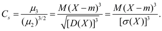
Third central point p 3 serves to characterize the asymmetry (skewness) of the distribution. It has the dimension of a random cube. To obtain a dimensionless value, it is divided by o 3, where a is the average standard deviation random variable X. The resulting value A called asymmetry coefficient of a random variable.
If the distribution is symmetrical relative to the mathematical expectation, then the asymmetry coefficient A = 0.
In Fig. Figure 3.17 shows two distribution curves: I and II. Curve I has a positive (right-sided) asymmetry (L > 0), and curve II has a negative (left-sided) asymmetry (L 

Fourth central point p 4 serves to characterize the steepness (sharpness or flatness) of the distribution.
Among the numerical characteristics of random variables, it is necessary, first of all, to note those that characterize the position of the random variable on the numerical axis, i.e. indicate some average, approximate value around which all possible values of a random variable are grouped.
The average value of a random variable is a certain number that is, as it were, its “representative” and replaces it in roughly approximate calculations. When we say: “the average lamp operating time is 100 hours” or “the average point of impact is shifted relative to the target by 2 m to the right,” we are indicating a certain numerical characteristic of a random variable that describes its location on the numerical axis, i.e. "position characteristics".
From the characteristics of position in probability theory vital role plays the mathematical expectation of a random variable, which is sometimes called simply the average value of the random variable.
Let's consider a discrete random variable having possible values with probabilities. We need to characterize with some number the position of the values of a random variable on the x-axis, taking into account the fact that these values have different probabilities. For this purpose, it is natural to use the so-called “weighted average” of the values, and each value during averaging should be taken into account with a “weight” proportional to the probability of this value. Thus, we will calculate the average of the random variable, which we will denote by:

or, given that,
 . (5.6.1)
This weighted average is called the mathematical expectation of the random variable. Thus, we introduced into consideration one of the most important concepts probability theory - the concept of mathematical expectation.
The mathematical expectation of a random variable is the sum of the products of all possible values of a random variable and the probabilities of these values.
Note that in the above formulation the definition of mathematical expectation is valid, strictly speaking, only for discrete random variables; Below we will generalize this concept to the case of continuous quantities.
In order to make the concept of mathematical expectation more clear, let us turn to the mechanical interpretation of the distribution of a discrete random variable. Let there be points with abscissas on the abscissa axis, in which the masses are concentrated, respectively, and . Then, obviously, the mathematical expectation defined by formula (5.6.1) is nothing more than the abscissa of the center of gravity of a given system of material points.
The mathematical expectation of a random variable is connected by a peculiar dependence with the arithmetic mean of the observed values of the random variable at large number experiments. This dependence is of the same type as the dependence between frequency and probability, namely: with a large number of experiments, the arithmetic mean of the observed values of a random variable approaches (converges in probability) to its mathematical expectation. From the presence of a connection between frequency and probability, one can deduce as a consequence the presence of a similar connection between the arithmetic mean and the mathematical expectation.
Indeed, consider a discrete random variable characterized by a distribution series:

Where ![]() .
.
Let independent experiments be carried out, in each of which the quantity takes a certain value. Let's assume that the value appeared once, the value appeared once, and the value appeared once. Obviously,
Let us calculate the arithmetic mean of the observed values of the quantity, which, in contrast to the mathematical expectation, we denote:
But there is nothing more than the frequency (or statistical probability) of an event; this frequency can be designated . Then
 ,
,
those. the arithmetic mean of the observed values of a random variable is equal to the sum of the products of all possible values of the random variable and the frequencies of these values.
As the number of experiments increases, the frequencies will approach (converge in probability) to the corresponding probabilities. Consequently, the arithmetic mean of the observed values of a random variable will approach (converge in probability) to its mathematical expectation as the number of experiments increases.
The connection between the arithmetic mean and mathematical expectation formulated above constitutes the content of one of the forms of the law large numbers. We will give a rigorous proof of this law in Chapter 13.
We already know that all forms of the law of large numbers state the fact that some averages are stable over a large number of experiments. Here we're talking about on the stability of the arithmetic mean from a series of observations of the same quantity. With a small number of experiments, the arithmetic mean of their results is random; with a sufficient increase in the number of experiments, it becomes “almost non-random” and, stabilizing, approaches constant value– mathematical expectation.
The stability of averages over a large number of experiments can be easily verified experimentally. For example, when weighing a body in a laboratory precise scales, as a result of weighing, we get a new value each time; To reduce observation error, we weigh the body several times and use the arithmetic mean of the obtained values. It is easy to see that with a further increase in the number of experiments (weighings), the arithmetic mean reacts to this increase less and less and, with a sufficiently large number of experiments, practically ceases to change.
Formula (5.6.1) for the mathematical expectation corresponds to the case of a discrete random variable. For continuous value the mathematical expectation, naturally, is expressed not as a sum, but as an integral:
 , (5.6.2)
where is the distribution density of the quantity .
Formula (5.6.2) is obtained from formula (5.6.1) if we replace it individual values continuously changing parameter x, the corresponding probabilities are the probability element, final amount– integral. In the future, we will often use this method of extending the formulas derived for discontinuous quantities to the case of continuous quantities.
In the mechanical interpretation, the mathematical expectation of a continuous random variable retains the same meaning - the abscissa of the center of gravity in the case when the mass is distributed along the abscissa continuously, with density . This interpretation often allows one to find the mathematical expectation without calculating the integral (5.6.2), from simple mechanical considerations.
Above we introduced a notation for the mathematical expectation of the quantity . In a number of cases, when a quantity is included in formulas as a specific number, it is more convenient to denote it by one letter. In these cases, we will denote the mathematical expectation of a value by:
The notations and for the mathematical expectation will be used in parallel in the future, depending on the convenience of a particular recording of the formulas. Let us also agree, if necessary, to abbreviate the words “mathematical expectation” with the letters m.o.
It should be noted that the most important characteristic of a position - the mathematical expectation - does not exist for all random variables. It is possible to compose examples of such random variables for which the mathematical expectation does not exist, since the corresponding sum or integral diverges.
Consider, for example, a discontinuous random variable with a distribution series:

It is easy to verify that, i.e. the distribution series makes sense; however the amount in in this case diverges and, therefore, there is no mathematical expectation of the value. However, such cases are not of significant interest for practice. Typically the random variables we deal with have limited area possible values and, of course, have a mathematical expectation.
Above we gave formulas (5.6.1) and (5.6.2), expressing the mathematical expectation, respectively, for a discontinuous and continuous random variable.
If the quantity belongs to the quantities mixed type, then its mathematical expectation is expressed by a formula of the form:
 , (5.6.3)
where the sum extends to all points at which the distribution function is discontinuous, and the integral extends to all areas at which the distribution function is continuous.
In addition to the most important of the characteristics of a position - the mathematical expectation - in practice, other characteristics of the position are sometimes used, in particular, the mode and median of a random variable.
The mode of a random variable is its most probable value. The term "most probable value" strictly speaking applies only to discontinuous quantities; for a continuous quantity, the mode is the value at which the probability density is maximum. Let us agree to denote the mode by the letter . In Fig. 5.6.1 and 5.6.2 show the mode for discontinuous and continuous random variables, respectively.


If the distribution polygon (distribution curve) has more than one maximum, the distribution is called “multimodal” (Fig. 5.6.3 and 5.6.4).


Sometimes there are distributions that have a minimum in the middle rather than a maximum (Fig. 5.6.5 and 5.6.6). Such distributions are called “anti-modal”. An example of an antimodal distribution is the distribution obtained in Example 5, n° 5.1.


IN general case the mode and mathematical expectation of a random variable do not coincide. In the particular case, when the distribution is symmetrical and modal (i.e. has a mode) and there is a mathematical expectation, then it coincides with the mode and center of symmetry of the distribution.
Another position characteristic is often used - the so-called median of a random variable. This characteristic is usually used only for continuous random variables, although it can be formally defined for a discontinuous variable.
The median of a random variable is its value for which
those. it is equally likely that the random variable will be less than or greater than . Geometrically, the median is the abscissa of the point at which the area limited by the distribution curve is divided in half (Fig. 5.6.7).
Expected value. Mathematical expectation discrete random variable X, host final number values Xi with probabilities Ri, the amount is called:
Mathematical expectation continuous random variable X is called the integral of the product of its values X on the probability distribution density f(x):
 (6b)
(6b)
Improper integral (6 b) is assumed to be absolutely convergent (in otherwise they say that the mathematical expectation M(X) does not exist). The mathematical expectation characterizes average value random variable X. Its dimension coincides with the dimension of the random variable.
Properties of mathematical expectation:
Dispersion. Variance random variable X the number is called:
The variance is scattering characteristic random variable values X relative to its average value M(X). The dimension of variance is equal to the dimension of the random variable squared. Based on the definitions of variance (8) and mathematical expectation (5) for a discrete random variable and (6) for a continuous random variable, we obtain similar expressions for the variance:
 (9)
(9)
Here m = M(X).
Dispersion properties:
Standard deviation:
![]() (11)
(11)
Since the dimension of the average square deviation the same as that of a random variable, it is more often used as a measure of dispersion than variance.
Moments of distribution. The concepts of mathematical expectation and dispersion are special cases of more general concept for numerical characteristics of random variables – distribution moments. The moments of distribution of a random variable are introduced as mathematical expectations of some simple functions of a random variable. So, moment of order k relative to the point X 0 is called the mathematical expectation M(X–X 0 )k. Moments about the origin X= 0 are called initial moments and are designated:
![]() (12)
(12)
The initial moment of the first order is the center of the distribution of the random variable under consideration:
![]() (13)
(13)
Moments about the center of distribution X= m are called central points and are designated:
![]() (14)
(14)
From (7) it follows that the first-order central moment is always equal to zero:
The central moments do not depend on the origin of the values of the random variable, since when shifted by constant value WITH its distribution center shifts by the same value WITH, and the deviation from the center does not change: X – m = (X – WITH) – (m – WITH).
Now it's obvious that dispersion- This second order central moment:
Asymmetry. Third order central moment:
![]() (17)
(17)
serves for evaluation distribution asymmetries. If the distribution is symmetrical about the point X= m, then the third-order central moment will be equal to zero (like all central moments of odd orders). Therefore, if the third-order central moment is different from zero, then the distribution cannot be symmetric. The magnitude of asymmetry is assessed using a dimensionless asymmetry coefficient:
 (18)
(18)
The sign of the asymmetry coefficient (18) indicates right-sided or left-sided asymmetry (Fig. 2).

Rice. 2. Types of distribution asymmetry.
Excess. Fourth order central moment:
![]() (19)
(19)
serves to evaluate the so-called excess, which determines the degree of steepness (pointedness) of the distribution curve near the center of the distribution in relation to the curve normal distribution. Since for a normal distribution, the value taken as kurtosis is:
 (20)
(20)
In Fig. 3 shows examples of distribution curves with different meanings excess. For normal distribution E= 0. Curves that are more pointed than normal have a positive kurtosis, those that are more flat-topped have a negative kurtosis.

Rice. 3. Distribution curves with varying degrees coolness (excess).
Higher-order moments in engineering applications mathematical statistics usually not used.
Fashion
discrete a random variable is its most probable value. Fashion continuous a random variable is its value at which the probability density is maximum (Fig. 2). If the distribution curve has one maximum, then the distribution is called unimodal. If a distribution curve has more than one maximum, then the distribution is called multimodal. Sometimes there are distributions whose curves have a minimum rather than a maximum. Such distributions are called anti-modal. In the general case, the mode and mathematical expectation of a random variable do not coincide. In the special case, for modal, i.e. having a mode, symmetrical distribution and provided that there is a mathematical expectation, the latter coincides with the mode and center of symmetry of the distribution.
Median random variable X- this is its meaning Meh, for which equality holds: i.e. it is equally probable that the random variable X will be less or more Meh. Geometrically median is the abscissa of the point at which the area under the distribution curve is divided in half (Fig. 2). In the case of a symmetric modal distribution, the median, mode and mathematical expectation are the same.