Standard deviation formula. Standard deviation of formula in excel

$X$. To begin with, let us recall the following definition:

Definition 1

Population-- a set of randomly selected objects of a given type, over which observations are carried out in order to obtain specific values of a random variable, carried out under constant conditions when studying one random variable of a given type.

Definition 2

General variance-- the arithmetic mean of the squared deviations of the values of the population variant from their mean value.

Let the values of option $x_1,\ x_2,\dots ,x_k$ have, respectively, frequencies $n_1,\ n_2,\dots ,n_k$. Then the general variance is calculated using the formula:

Let's consider a special case. Let all options $x_1,\ x_2,\dots ,x_k$ be different. In this case $n_1,\ n_2,\dots ,n_k=1$. We find that in this case the general variance is calculated using the formula:

This concept is also associated with the concept of general standard deviation.

Definition 3

General standard deviation

\[(\sigma )_g=\sqrt(D_g)\]

Sample variance

Let us be given a sample population with respect to a random variable $X$. To begin with, let us recall the following definition:

Definition 4

Sample population-- part of selected objects from the general population.

Definition 5

Sample variance-- arithmetic mean of the values of the sample population.

Let the values of option $x_1,\ x_2,\dots ,x_k$ have, respectively, frequencies $n_1,\ n_2,\dots ,n_k$. Then the sample variance is calculated using the formula:

Let's consider a special case. Let all options $x_1,\ x_2,\dots ,x_k$ be different. In this case $n_1,\ n_2,\dots ,n_k=1$. We find that in this case the sample variance is calculated by the formula:

Also related to this concept is the concept of sample standard deviation.

Definition 6

Sample standard deviation-- square root of the general variance:

\[(\sigma )_в=\sqrt(D_в)\]

Corrected variance

To find the corrected variance $S^2$ it is necessary to multiply the sample variance by the fraction $\frac(n)(n-1)$, that is

This concept is also associated with the concept of corrected standard deviation, which is found by the formula:

In the case when the values of the variants are not discrete, but represent intervals, then in the formulas for calculating the general or sample variances, the value of $x_i$ is taken to be the value of the middle of the interval to which $x_i.$ belongs.

An example of a problem to find the variance and standard deviation

Example 1

The sample population is defined by the following distribution table:

Picture 1.

Let us find for it the sample variance, sample standard deviation, corrected variance and corrected standard deviation.

To solve this problem, we first make a calculation table:

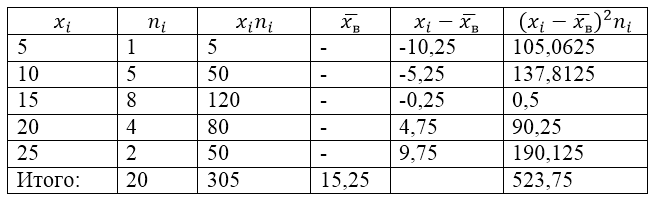
Figure 2.

The value $\overline(x_в)$ (sample average) in the table is found by the formula:

\[\overline(x_in)=\frac(\sum\limits^k_(i=1)(x_in_i))(n)\]

\[\overline(x_in)=\frac(\sum\limits^k_(i=1)(x_in_i))(n)=\frac(305)(20)=15.25\]

Let's find the sample variance using the formula:

Sample standard deviation:

\[(\sigma )_в=\sqrt(D_в)\approx 5.12\]

Corrected variance:

\[(S^2=\frac(n)(n-1)D)_в=\frac(20)(19)\cdot 26.1875\approx 27.57\]

Corrected standard deviation.

Standard deviation(synonyms: standard deviation, standard deviation, square deviation; related terms: standard deviation, standard spread) - in probability theory and statistics, the most common indicator of the dispersion of the values of a random variable relative to its mathematical expectation. With limited arrays of samples of values, instead of the mathematical expectation, the arithmetic mean of the set of samples is used.

Encyclopedic YouTube

1 / 5
The standard deviation is measured in units of measurement of the random variable itself and is used when calculating the standard error of the arithmetic mean, when constructing confidence intervals, when statistically testing hypotheses, when measuring the linear relationship between random variables. Defined as the square root of the variance of a random variable.
Standard deviation:
s = n n − 1 σ 2 = 1 n − 1 ∑ i = 1 n (x i − x ¯) 2 ; (\displaystyle s=(\sqrt ((\frac (n)(n-1))\sigma ^(2)))=(\sqrt ((\frac (1)(n-1))\sum _( i=1)^(n)\left(x_(i)-(\bar (x))\right)^(2)));)
- Note: Very often there are discrepancies in the names of MSD (Root Mean Square Deviation) and STD (Standard Deviation) with their formulas. For example, in the numPy module of the Python programming language, the std() function is described as "standard deviation", while the formula reflects the standard deviation (division by the root of the sample). In Excel, the STANDARDEVAL() function is different (division by the root of n-1).
Standard deviation(estimate of the standard deviation of a random variable x relative to its mathematical expectation based on an unbiased estimate of its variance) s (\displaystyle s):
σ = 1 n ∑ i = 1 n (x i − x ¯) 2 . (\displaystyle \sigma =(\sqrt ((\frac (1)(n))\sum _(i=1)^(n)\left(x_(i)-(\bar (x))\right) ^(2))).)
Where σ 2 (\displaystyle \sigma ^(2))- dispersion; x i (\displaystyle x_(i)) - i th element of the selection; n (\displaystyle n)- sample size; - arithmetic mean of the sample:
x ¯ = 1 n ∑ i = 1 n x i = 1 n (x 1 + … + x n) . (\displaystyle (\bar (x))=(\frac (1)(n))\sum _(i=1)^(n)x_(i)=(\frac (1)(n))(x_ (1)+\ldots +x_(n)).)
It should be noted that both estimates are biased. In the general case, it is impossible to construct an unbiased estimate. However, the estimate based on the unbiased variance estimate is consistent.
In accordance with GOST R 8.736-2011, the standard deviation is calculated using the second formula of this section. Please check the results.

Three sigma rule

Three sigma rule (3 σ (\displaystyle 3\sigma )) - almost all values of a normally distributed random variable lie in the interval (x ¯ − 3 σ ; x ¯ + 3 σ) (\displaystyle \left((\bar (x))-3\sigma ;(\bar (x))+3\sigma \right)). More strictly - with approximately probability 0.9973, the value of a normally distributed random variable lies in the specified interval (provided that the value x ¯ (\displaystyle (\bar (x))) true, and not obtained as a result of sample processing).
If the true value x ¯ (\displaystyle (\bar (x))) is unknown, then you should not use σ (\displaystyle \sigma ), A s. Thus, the rule of three sigma is transformed into the rule of three s .

Interpretation of the standard deviation value

A larger standard deviation value shows a greater spread of values in the presented set with the average value of the set; a smaller value, accordingly, shows that the values in the set are grouped around the average value.
For example, we have three number sets: (0, 0, 14, 14), (0, 6, 8, 14) and (6, 6, 8, 8). All three sets have mean values equal to 7, and standard deviations, respectively, equal to 7, 5 and 1. The last set has a small standard deviation, since the values in the set are grouped around the mean value; the first set has the largest standard deviation value - the values within the set diverge greatly from the average value.
In a general sense, standard deviation can be considered a measure of uncertainty. For example, in physics, standard deviation is used to determine the error of a series of successive measurements of some quantity. This value is very important for determining the plausibility of the phenomenon under study in comparison with the value predicted by the theory: if the average value of the measurements differs greatly from the values predicted by the theory (large standard deviation), then the obtained values or the method of obtaining them should be rechecked. identified with portfolio risk.

Climate

Suppose there are two cities with the same average maximum daily temperature, but one is located on the coast and the other on the plain. It is known that cities located on the coast have many different maximum daytime temperatures that are lower than cities located inland. Therefore, the standard deviation of the maximum daily temperatures for a coastal city will be less than for the second city, despite the fact that the average value of this value is the same, which in practice means that the probability that the maximum air temperature on any given day of the year will be higher differ from the average value, higher for a city located inland.

Sport

Let's assume that there are several football teams that are rated on some set of parameters, for example, the number of goals scored and conceded, scoring chances, etc. It is most likely that the best team in this group will have better values on more parameters. The smaller the team’s standard deviation for each of the presented parameters, the more predictable the team’s result is; such teams are balanced. On the other hand, a team with a large standard deviation is difficult to predict the result, which in turn is explained by an imbalance, for example, a strong defense but a weak attack.
Using the standard deviation of team parameters makes it possible, to one degree or another, to predict the result of a match between two teams, assessing the strengths and weaknesses of the teams, and therefore the chosen methods of fighting.

Standard deviation

The most perfect characteristic of variation is the mean square deviation, which is called the standard (or standard deviation). Standard deviation() is equal to the square root of the average square deviation of individual values of the attribute from the arithmetic mean:

The standard deviation is simple:

Weighted standard deviation is applied to grouped data:

The following ratio takes place between the mean square and mean linear deviations under normal distribution conditions: ~ 1.25.

The standard deviation, being the main absolute measure of variation, is used in determining the ordinate values of a normal distribution curve, in calculations related to the organization of sample observation and establishing the accuracy of sample characteristics, as well as in assessing the limits of variation of a characteristic in a homogeneous population.

18. Variance, its types, standard deviation.

Variance of a random variable- a measure of the spread of a given random variable, i.e. its deviation from the mathematical expectation. In statistics, the notation or is often used. The square root of the variance is usually called standard deviation, standard deviation or standard spread.

Total variance (σ 2) measures the variation of a trait in its entirety under the influence of all the factors that caused this variation. At the same time, thanks to the grouping method, it is possible to identify and measure the variation due to the grouping characteristic and the variation arising under the influence of unaccounted factors.

Intergroup variance (σ 2 m.gr) characterizes systematic variation, i.e. differences in the value of the studied trait that arise under the influence of the trait - the factor that forms the basis of the group.

Standard deviation(synonyms: standard deviation, standard deviation, square deviation; related terms: standard deviation, standard spread) - in probability theory and statistics, the most common indicator of the dispersion of the values of a random variable relative to its mathematical expectation. With limited arrays of samples of values, instead of the mathematical expectation, the arithmetic mean of the set of samples is used.

The standard deviation is measured in units of measurement of the random variable itself and is used when calculating the standard error of the arithmetic mean, when constructing confidence intervals, when statistically testing hypotheses, when measuring the linear relationship between random variables. Defined as the square root of the variance of a random variable.

Standard deviation:

Standard deviation(estimate of the standard deviation of a random variable x relative to its mathematical expectation based on an unbiased estimate of its variance):

where is the dispersion; - i th element of the selection; - sample size; - arithmetic mean of the sample:

It should be noted that both estimates are biased. In the general case, it is impossible to construct an unbiased estimate. In this case, the estimate based on the unbiased variance estimate is consistent.

19. Essence, scope and procedure for determining mode and median.

In addition to power averages in statistics, for the relative characterization of the value of a varying characteristic and the internal structure of distribution series, structural averages are used, which are represented mainly by fashion and median.

Fashion- This is the most common variant of the series. Fashion is used, for example, in determining the size of clothes and shoes that are in greatest demand among customers. The mode for a discrete series is the variant with the highest frequency. When calculating the mode for an interval variation series, it is extremely important to first determine the modal interval (by maximum frequency), and then - the value of the modal value of the attribute using the formula:

§ - meaning of fashion

§ - lower limit of the modal interval

§ - interval value

§ - modal interval frequency

§ - frequency of the interval preceding the modal

§ - frequency of the interval following the modal

Median - this value of the attribute, ĸᴏᴛᴏᴩᴏᴇ lies in the basis of the ranked series and divides this series into two parts equal in number.

To determine the median in a discrete series if frequencies are available, first calculate the half-sum of frequencies , and then determine which value of the variant falls on it. (If the sorted series contains an odd number of characteristics, then the median number is calculated using the formula:

M e = (n (number of features in total) + 1)/2,

in the case of an even number of features, the median will be equal to the average of the two features in the middle of the row).

When calculating the median for interval variation series First, determine the median interval within which the median is located, and then determine the value of the median using the formula:

§ - the required median

§ - lower limit of the interval that contains the median

§ - interval value

§ - sum of frequencies or number of series terms

§ - the sum of the accumulated frequencies of the intervals preceding the median

§ - frequency of the median interval

Example. Find the mode and median.

Solution: In this example, the modal interval is within the age group of 25-30 years, since this interval has the highest frequency (1054).

Let's calculate the magnitude of the mode:

This means that the modal age of students is 27 years.

Let's calculate the median. The median interval is in the age group of 25-30 years, since within this interval there is an option͵ which divides the population into two equal parts (Σf i /2 = 3462/2 = 1731). Next, we substitute the necessary numerical data into the formula and get the median value:

This means that one half of the students are under 27.4 years old, and the other half are over 27.4 years old.

In addition to mode and median, indicators such as quartiles are used, dividing the ranked series into 4 equal parts, deciles - 10 parts and percentiles - into 100 parts.

20. The concept of sample observation and its scope.

Selective observation applies when the use of continuous surveillance physically impossible due to a large amount of data or not economically feasible. Physical impossibility occurs, for example, when studying passenger flows, market prices, and family budgets. Economic inexpediency occurs when assessing the quality of goods associated with their destruction, for example, tasting, testing bricks for strength, etc.

The statistical units selected for observation are sample population or sample, and their entire array - general population(GS). Wherein number of units in sample denote n, and in the entire GS - N. Attitude n/N usually called relative size or sample share.

The quality of sample observation results depends on sample representativeness, that is, on how representative it is in the GS. To ensure the representativeness of the sample, it is extremely important to comply principle of random selection of units, which assumes that the inclusion of a HS unit in the sample cannot be influenced by any factor other than chance.

Exists 4 ways of random selection to sample:
1. Actually random selection or the “lotto method”, when statistical values are assigned serial numbers, recorded on certain objects (for example, barrels), which are then mixed in a container (for example, in a bag) and selected at random. In practice, this method is carried out using a random number generator or mathematical tables of random numbers.
2. Mechanical selection according to which each ( N/n)-th value of the general population. For example, if it contains 100,000 values, and you need to select 1,000, then every 100,000 / 1000 = 100th value will be included in the sample. Moreover, if they are not ranked, then the first one is selected at random from the first hundred, and the numbers of the others will be one hundred higher. For example, if the first unit was No. 19, then the next should be No. 119, then No. 219, then No. 319, etc. If the population units are ranked, then No. 50 is selected first, then No. 150, then No. 250, and so on.
3. Selection of values from a heterogeneous data array is carried out stratified(stratified) method, when the population is first divided into homogeneous groups to which random or mechanical selection is applied.
4. A special sampling method is serial selection, in which they randomly or mechanically select not individual values, but their series (sequences from some number to some number in a row), within which continuous observation is carried out.
The quality of sample observations also depends on sample type: repeated or unrepeatable. At re-selection Statistical values or their series included in the sample are returned to the general population after use, having a chance to be included in a new sample. Moreover, all values in the general population have the same probability of inclusion in the sample. Repeatless selection means that the statistical values or their series included in the sample do not return to the general population after use, and therefore for the remaining values of the latter the probability of being included in the next sample increases.

Non-repetitive sampling gives more accurate results, and therefore is used more often. But there are situations when it cannot be applied (studying passenger flows, consumer demand, etc.) and then a repeated selection is carried out.

21. Maximum observation sampling error, average sampling error, procedure for their calculation.

Let us consider in detail the methods listed above for forming a sample population and the representativeness errors that arise. Properly random sampling is based on selecting units from the population at random without any systematic elements. Technically, actual random selection is carried out by drawing lots (for example, lotteries) or using a table of random numbers.

Proper random selection “in its pure form” is rarely used in the practice of selective observation, but it is the initial one among other types of selection; it implements the basic principles of selective observation. Let's consider some questions of the theory of the sampling method and the error formula for a simple random sample.

Sampling bias- ϶ᴛᴏ the difference between the value of the parameter in the general population and its value calculated from the results of sample observation. It is important to note that for the average quantitative characteristic the sampling error is determined by

The indicator is usually called the maximum sampling error. The sample mean is a random variable that can take on different values based on which units are included in the sample. Therefore, sampling errors are also random variables and can take on different values. For this reason, the average of possible errors is determined - average sampling error, which depends on:

· sample size: the larger the number, the smaller the average error;

· the degree of change in the characteristic being studied: the smaller the variation of the characteristic, and, consequently, the dispersion, the smaller the average sampling error.

At random re-selection the average error is calculated. In practice, the general variance is not known exactly, but in probability theory it has been proven that . Since the value for sufficiently large n is close to 1, we can assume that . Then the average sampling error should be calculated: . But in cases of a small sample (with n<30) коэффициент крайне важно учитывать, и среднюю ошибку малой выборки рассчитывать по формуле .

At random non-repetitive sampling the given formulas are adjusted by the value . Then the average non-repetitive sampling error is: And . Because is always less than , then the multiplier () is always less than 1. This means that the average error with repeated selection is always less than with repeated selection. Mechanical sampling is used when the general population is ordered in some way (for example, lists of voters in alphabetical order, telephone numbers, house and apartment numbers). The selection of units is carried out at a certain interval, which is equal to the inverse value of the sampling percentage. So, with a 2% sample, every 50 unit = 1/0.02 is selected, with a 5% sample, every 1/0.05 = 20 unit of the general population.

The reference point is selected in different ways: randomly, from the middle of the interval, with a change in the reference point. The main thing is to avoid systematic errors. For example, with a 5% sample, if the first unit is the 13th, then the next ones are 33, 53, 73, etc.

In terms of accuracy, mechanical selection is close to actual random sampling. For this reason, to determine the average error of mechanical sampling, proper random selection formulas are used.

At typical selection the population being surveyed is preliminarily divided into homogeneous, similar groups. For example, when surveying enterprises, these are industries, sub-sectors; when studying the population, these are regions, social or age groups. Next, an independent selection from each group is made mechanically or purely randomly.

Typical sampling produces more accurate results than other methods. Typing the general population ensures that each typological group is represented in the sample, which makes it possible to eliminate the influence of intergroup variance on the average sampling error. Therefore, when finding the error of a typical sample according to the rule of adding variances (), it is extremely important to take into account only the average of the group variances. Then the average sampling error: with repeated sampling, with non-repetitive sampling , Where – the average of the within-group variances in the sample.

Serial (or nest) selection used when the population is divided into series or groups before the start of the sample survey. These series include packaging of finished products, student groups, and brigades. Series for examination are selected mechanically or purely randomly, and within the series a continuous examination of units is carried out. For this reason, the average sampling error depends only on the intergroup (between series) variance, which is calculated using the formula: where r is the number of selected series; – average of the i-th series. The average error of serial sampling is calculated: with repeated sampling, with non-repetitive sampling , where R is the total number of series. Combined selection is a combination of the considered selection methods.

The average sampling error for any sampling method depends mainly on the absolute size of the sample and, to a lesser extent, on the percentage of the sample. Let us assume that 225 observations are made in the first case from a population of 4,500 units and in the second from a population of 225,000 units. The variances in both cases are equal to 25. Then in the first case, with a 5% selection, the sampling error will be: In the second case, with 0.1% selection, it will be equal to:

However, when the sampling percentage was reduced by 50 times, the sampling error increased slightly, since the sample size did not change. Let's assume that the sample size is increased to 625 observations. In this case, the sampling error is: Increasing the sample by 2.8 times with the same population size reduces the size of the sampling error by more than 1.6 times.

22.Methods and methods for forming a sample population.

In statistics, various methods of forming sample populations are used, which is determined by the objectives of the study and depends on the specifics of the object of study.

The main condition for conducting a sample survey is to prevent the occurrence of systematic errors arising from violation of the principle of equal opportunity for each unit of the general population to be included in the sample. Prevention of systematic errors is achieved through the use of scientifically based methods for forming a sample population.

There are the following methods for selecting units from the general population: 1) individual selection - individual units are selected for the sample; 2) group selection - the sample includes qualitatively homogeneous groups or series of units being studied; 3) combined selection is a combination of individual and group selection. Selection methods are determined by the rules for forming a sample population.

The sample should be:
- actually random consists in the fact that the sample population is formed as a result of random (unintentional) selection of individual units from the general population. In this case, the number of units selected in the sample population is usually determined based on the accepted sample proportion. The sample proportion is the ratio of the number of units in the sample population n to the number of units in the general population N, ᴛ.ᴇ.
- mechanical consists in the fact that the selection of units in the sample population is made from the general population, divided into equal intervals (groups). In this case, the size of the interval in the population is equal to the reciprocal of the sample share. So, with a 2% sample, every 50th unit is selected (1:0.02), with a 5% sample, every 20th unit (1:0.05), etc. However, in accordance with the accepted proportion of selection, the general population is, as it were, mechanically divided into equal groups. From each group, only one unit is selected for the sample.
- typical – in which the general population is first divided into homogeneous typical groups. Next, from each typical group, a purely random or mechanical sample is used to individually select units into the sample population. An important feature of a typical sample is that it gives more accurate results compared to other methods of selecting units in the sample population;
- serial- in which the general population is divided into groups of equal size - series. Series are selected into the sample population. Within the series, continuous observation of the units included in the series is carried out;
- combined- sampling should be two-stage. In this case, the population is first divided into groups. Next, groups are selected, and within the latter, individual units are selected.
In statistics, the following methods are distinguished for selecting units in a sample population:
- single stage sampling - each selected unit is immediately subjected to study according to a given criterion (proper random and serial sampling);
- multi-stage sampling - a selection is made from the general population of individual groups, and individual units are selected from the groups (typical sampling with a mechanical method of selecting units into the sample population).
In addition, there are:
- re-selection- according to the scheme of the returned ball. In this case, each unit or series included in the sample is returned to the general population and therefore has a chance to be included in the sample again;
- repeat selection- according to the unreturned ball scheme. It has more accurate results with the same sample size.
23. Determination of the extremely important sample size (using the Student's t-table).

One of the scientific principles in sampling theory is to ensure that a sufficient number of units are selected. Theoretically, the extreme importance of observing this principle is presented in the proofs of limit theorems in probability theory, which make it possible to establish what volume of units should be selected from the population so that it is sufficient and ensures the representativeness of the sample.

A decrease in the standard sampling error, and therefore an increase in the accuracy of the estimate, is always associated with an increase in the sample size; therefore, already at the stage of organizing a sample observation, it is necessary to decide what the size of the sample population should be in order to ensure the required accuracy of the observation results . The calculation of the extremely important sample volume is constructed using formulas derived from the formulas for the maximum sampling errors (A), corresponding to a particular type and method of selection. So, for a random repeated sample size (n) we have:

The essence of this formula is that with random repeated sampling of extremely important numbers, the sample size is directly proportional to the square of the confidence coefficient (t2) and variance of the variational characteristic (?2) and is inversely proportional to the square of the maximum sampling error (?2). In particular, with an increase in the maximum error by a factor of two, the required sample size should be reduced by a factor of four. Of the three parameters, two (t and?) are set by the researcher. At the same time, the researcher, based on the goal

and the problems of a sample survey must solve the question: in what quantitative combination is it better to include these parameters to ensure the optimal option? In one case, he may be more satisfied with the reliability of the results obtained (t) than with the measure of accuracy (?), in another - vice versa. It is more difficult to resolve the issue regarding the value of the maximum sampling error, since the researcher does not have this indicator at the stage of designing the sample observation; therefore, in practice it is customary to set the value of the maximum sampling error, usually within 10% of the expected average level of the attribute . Establishing the estimated average can be approached in different ways: using data from similar previous surveys, or using data from the sampling frame and conducting a small pilot sample.

The most difficult thing to establish when designing a sample observation is the third parameter in formula (5.2) - the variance of the sample population. In this case, it is extremely important to use all the information available to the researcher, obtained in previous similar and pilot surveys.

The question of determining the extremely important sample size becomes more complicated if the sample survey involves the study of several characteristics of sampling units. In this case, the average levels of each of the characteristics and their variation, as a rule, are different, and in this regard, deciding which variance of which of the characteristics to give preference to is possible only taking into account the purpose and objectives of the survey.

When designing a sample observation, a predetermined value of the permissible sampling error is assumed in accordance with the objectives of a particular study and the probability of conclusions based on the observation results.

In general, the formula for the maximum error of the sample average allows us to determine:

‣‣‣ the magnitude of possible deviations of the indicators of the general population from the indicators of the sample population;

‣‣‣ the required sample size to ensure the required accuracy, at which the limits of possible error do not exceed a certain specified value;

‣‣‣ the probability that the error in the sample will have a specified limit.

Student distribution in probability theory, it is a one-parameter family of absolutely continuous distributions.

24. Dynamic series (interval, moment), closing dynamic series.

Dynamics series- these are the values of statistical indicators that are presented in a certain chronological sequence.

Each time series contains two components:

1) indicators of time periods(years, quarters, months, days or dates);

2) indicators characterizing the object under study for time periods or on corresponding dates, which are called series levels.

Series levels are expressed in both absolute and average or relative values. Taking into account the dependence on the nature of the indicators, dynamic series of absolute, relative and average values are built. Dynamic series of relative and average values are constructed on the basis of derived series of absolute values. There are interval and moment series of dynamics.

Dynamic interval series contains the values of indicators for certain periods of time. In an interval series, levels can be summed up to obtain the volume of the phenomenon over a longer period, or the so-called accumulated totals.

Dynamic moment series reflects the values of indicators at a certain point in time (date of time). In moment series, the researcher may only be interested in the difference in phenomena that reflects the change in the level of the series between certain dates, since the sum of the levels here has no real content. Cumulative totals are not calculated here.

The most important condition for the correct construction of time series is comparability of series levels belonging to different periods. The levels must be presented in homogeneous quantities, and there must be equal completeness of coverage of different parts of the phenomenon.

In order to avoid distortion of the real dynamics, in statistical research preliminary calculations are carried out (closing the dynamics series), which precede the statistical analysis of the time series. Under closing the series of dynamics It is generally accepted to understand the combination into one series of two or more series, the levels of which are calculated using different methodology or do not correspond to territorial boundaries, etc. Closing the dynamics series may also imply bringing the absolute levels of the dynamics series to a common basis, which neutralizes the incomparability of the levels of the dynamics series.

25. The concept of comparability of dynamics series, coefficients, growth and growth rates.

Dynamics series- these are a series of statistical indicators characterizing the development of natural and social phenomena over time. Statistical collections published by the State Statistics Committee of Russia contain a large number of dynamics series in tabular form. Dynamic series make it possible to identify patterns of development of the phenomena being studied.

Dynamics series contain two types of indicators. Time indicators(years, quarters, months, etc.) or points in time (at the beginning of the year, at the beginning of each month, etc.). Row level indicators. Indicators of the levels of dynamics series can be expressed in absolute values (product production in tons or rubles), relative values (share of the urban population in %) and average values (average salary of industry workers by year, etc.). In tabular form, a time series contains two columns or two rows.

Correct construction of time series requires the fulfillment of a number of requirements:
1. all indicators of a number of dynamics must be scientifically substantiated and reliable;
2. indicators of a series of dynamics must be comparable over time, ᴛ.ᴇ. must be calculated for the same periods of time or on the same dates;
3. indicators of a number of dynamics must be comparable across the territory;
4. indicators of a series of dynamics must be comparable in content, ᴛ.ᴇ. calculated according to a single methodology, in the same way;
5. indicators of a number of dynamics should be comparable across the range of farms taken into account. All indicators of a series of dynamics must be given in the same units of measurement.
Statistical indicators can characterize either the results of the process being studied over a period of time, or the state of the phenomenon being studied at a certain point in time, ᴛ.ᴇ. indicators can be interval (periodic) and momentary. Accordingly, initially the dynamics series are either interval or moment. Moment dynamics series, in turn, come with equal and unequal time intervals.

The original dynamics series can be transformed into a series of average values and a series of relative values (chain and basic). Such time series are called derived time series.

The methodology for calculating the average level in the dynamics series is different, depending on the type of the dynamics series. Using examples, we will consider the types of dynamics series and formulas for calculating the average level.

Absolute increases (Δy) show how many units the subsequent level of the series has changed compared to the previous one (gr. 3. - chain absolute increases) or compared to the initial level (gr. 4. - basic absolute increases). The calculation formulas can be written as follows:

When the absolute values of the series decrease, there will be a “decrease” or “decrease”, respectively.

Absolute growth indicators indicate that, for example, in 1998. production of product "A" increased compared to 1997. by 4 thousand tons, and compared to 1994 ᴦ. - by 34 thousand tons; for other years, see table. 11.5 gr.
Posted on ref.rf
3 and 4.

Growth rate shows how many times the level of the series has changed compared to the previous one (gr. 5 - chain coefficients of growth or decline) or compared to the initial level (gr. 6 - basic coefficients of growth or decline). The calculation formulas can be written as follows:

Rates of growth show what percentage the next level of the series is compared to the previous one (gr. 7 - chain growth rates) or compared to the initial level (gr. 8 - basic growth rates). The calculation formulas can be written as follows:

So, for example, in 1997. production volume of product "A" compared to 1996 ᴦ. amounted to 105.5% (

Growth rate show by what percentage the level of the reporting period increased compared to the previous one (column 9 - chain growth rates) or compared to the initial level (column 10 - basic growth rates). The calculation formulas can be written as follows:

T pr = T r - 100% or T pr = absolute growth / level of the previous period * 100%

So, for example, in 1996. compared to 1995 ᴦ. Product "A" was produced more by 3.8% (103.8% - 100%) or (8:210)x100%, and compared to 1994 ᴦ. - by 9% (109% - 100%).

If the absolute levels in the series decrease, then the rate will be less than 100% and, accordingly, there will be a rate of decrease (the rate of increase with a minus sign).

Absolute value of 1% increase(gr.
Posted on ref.rf
11) shows how many units need to be produced in a given period so that the level of the previous period increases by 1%. In our example, in 1995 ᴦ. it was necessary to produce 2.0 thousand tons, and in 1998 ᴦ. - 2.3 thousand tons, ᴛ.ᴇ. much bigger.

The absolute value of 1% growth can be determined in two ways:

§ the level of the previous period divided by 100;

§ chain absolute increases are divided by the corresponding chain growth rates.

Absolute value of 1% increase =

In dynamics, especially over a long period, a joint analysis of the growth rate with the content of each percentage increase or decrease is important.

Note that the considered methodology for analyzing time series is applicable both for time series, the levels of which are expressed in absolute values (t, thousand rubles, number of employees, etc.), and for time series, the levels of which are expressed in relative indicators (% of defects , % ash content of coal, etc.) or average values (average yield in c/ha, average salary, etc.).

Along with the considered analytical indicators, calculated for each year in comparison with the previous or initial level, when analyzing dynamics series, it is extremely important to calculate the average analytical indicators for the period: the average level of the series, the average annual absolute increase (decrease) and the average annual growth rate and growth rate .

Methods for calculating the average level of a series of dynamics were discussed above. In the interval dynamics series we are considering, the average level of the series is calculated using the simple arithmetic mean formula:

Average annual production volume of the product for 1994-1998. amounted to 218.4 thousand tons.

The average annual absolute growth is also calculated using the arithmetic mean formula

Standard deviation - concept and types. Classification and features of the category "Mean square deviation" 2017, 2018.

Lesson No. 4
Topic: “Descriptive statistics. Indicators of trait diversity in the aggregate"
The main criteria for the diversity of a characteristic in a statistical population are: limit, amplitude, standard deviation, coefficient of oscillation and coefficient of variation. In the previous lesson, it was discussed that average values provide only a generalized characteristic of the characteristic being studied in the aggregate and do not take into account the values of its individual variants: minimum and maximum values, above average, below average, etc.
Example. Average values of two different number sequences: -100; -20; 100; 20 and 0.1; -0.2; 0.1 are absolutely identical and equalABOUT.However, the scatter ranges of these relative mean sequence data are very different.
The determination of the listed criteria for the diversity of a characteristic is primarily carried out taking into account its value in individual elements of the statistical population.
Indicators for measuring variation of a trait are absolute And relative. Absolute indicators of variation include: range of variation, limit, standard deviation, dispersion. The coefficient of variation and the coefficient of oscillation refer to relative measures of variation.
Limit (lim)– This is a criterion that is determined by the extreme values of a variant in a variation series. In other words, this criterion is limited by the minimum and maximum values of the attribute:
Amplitude (Am) or range of variation – This is the difference between the extreme options. The calculation of this criterion is carried out by subtracting its minimum value from the maximum value of the attribute, which allows us to estimate the degree of scatter of the option:
The disadvantage of limit and amplitude as criteria of variability is that they completely depend on the extreme values of the characteristic in the variation series. In this case, fluctuations in attribute values within a series are not taken into account.
The most complete description of the diversity of a trait in a statistical population is provided by standard deviation(sigma), which is a general measure of the deviation of an option from its average value. Standard deviation is often called standard deviation.
The standard deviation is based on a comparison of each option with the arithmetic mean of a given population. Since in the aggregate there will always be options both less and more than it, the sum of deviations with the sign "" will be canceled out by the sum of deviations with the sign "", i.e. the sum of all deviations is zero. In order to avoid the influence of the signs of the differences, deviations from the arithmetic mean squared are taken, i.e. . The sum of squared deviations does not equal zero. To obtain a coefficient that can measure variability, take the average of the sum of squares - this value is called variances:
In essence, dispersion is the average square of deviations of individual values of a characteristic from its average value. Dispersion – square of the standard deviation.
Variance is a dimensional quantity (named). So, if the variants of a number series are expressed in meters, then the variance gives square meters; if the options are expressed in kilograms, then the variance gives the square of this measure (kg 2), etc.
Standard deviation– square root of variance:
, then when calculating the dispersion and standard deviation in the denominator of the fraction, instead ofmust be put.
The calculation of the standard deviation can be divided into six stages, which must be carried out in a certain sequence:
Application of standard deviation:
a) for judging the variability of variation series and comparative assessment of the typicality (representativeness) of arithmetic averages. This is necessary in differential diagnosis when determining the stability of symptoms.
b) to reconstruct the variation series, i.e. restoration of its frequency response based on three sigma rules. In the interval (М±3σ) 99.7% of all variants of the series are located in the interval (М±2σ) - 95.5% and in the range (М±1σ) - 68.3% row variant(Fig. 1).
c) to identify “pop-up” options
d) to determine the parameters of norm and pathology using sigma estimates
e) to calculate the coefficient of variation
f) to calculate the average error of the arithmetic mean.
To characterize any population that hasnormal distribution type , it is enough to know two parameters: the arithmetic mean and the standard deviation.
Figure 1. Three Sigma rule
Example.
In pediatrics, standard deviation is used to assess the physical development of children by comparing the data of a particular child with the corresponding standard indicators. The arithmetic average of the physical development of healthy children is taken as the standard. Comparison of indicators with standards is carried out using special tables in which the standards are given along with their corresponding sigma scales. It is believed that if the indicator of a child’s physical development is within the standard (arithmetic mean) ±σ, then the child’s physical development (according to this indicator) corresponds to the norm. If the indicator is within the standard ±2σ, then there is a slight deviation from the norm. If the indicator goes beyond these limits, then the child’s physical development differs sharply from the norm (pathology is possible).
In addition to variation indicators expressed in absolute values, statistical research uses variation indicators expressed in relative values. Oscillation coefficient - this is the ratio of the range of variation to the average value of the trait. The coefficient of variation - this is the ratio of the standard deviation to the average value of the characteristic. Typically, these values are expressed as percentages.
Formulas for calculating relative variation indicators:
From the above formulas it is clear that the greater the coefficient V is closer to zero, the smaller the variation in the values of the characteristic. The more V, the more variable the sign.
In statistical practice, the coefficient of variation is most often used. It is used not only for a comparative assessment of variation, but also to characterize the homogeneity of the population. The population is considered homogeneous if the coefficient of variation does not exceed 33% (for distributions close to normal). Arithmetically, the ratio of σ and the arithmetic mean neutralizes the influence of the absolute value of these characteristics, and the percentage ratio makes the coefficient of variation a dimensionless (unnamed) value.
The resulting value of the coefficient of variation is estimated in accordance with the approximate gradations of the degree of diversity of the trait:
Weak - up to 10%
Average - 10 - 20%
Strong - more than 20%
The use of the coefficient of variation is advisable in cases where it is necessary to compare characteristics that are different in size and dimension.
The difference between the coefficient of variation and other scatter criteria is clearly demonstrated example.
Table 1
Composition of industrial enterprise workers

Based on the statistical characteristics given in the example, we can draw a conclusion about the relative homogeneity of the age composition and educational level of the enterprise’s employees, given the low professional stability of the surveyed contingent. It is easy to see that an attempt to judge these social trends by the standard deviation would lead to an erroneous conclusion, and an attempt to compare the accounting characteristics “work experience” and “age” with the accounting indicator “education” would generally be incorrect due to the heterogeneity of these characteristics.
Median and percentiles
For ordinal (rank) distributions, where the criterion for the middle of the series is the median, the standard deviation and dispersion cannot serve as characteristics of the dispersion of the variant.
The same is true for open variation series. This circumstance is due to the fact that the deviations from which variance and σ are calculated are measured from the arithmetic mean, which is not calculated in open variation series and in series of distributions of qualitative characteristics. Therefore, for a compressed description of distributions, another scatter parameter is used - quantile(synonym - “percentile”), suitable for describing qualitative and quantitative characteristics in any form of their distribution. This parameter can also be used to convert quantitative characteristics into qualitative ones. In this case, such ratings are assigned depending on which order of quantile a particular option corresponds to.
In the practice of biomedical research, the following quantiles are most often used:
– median;
, – quartiles (quarters), where – lower quartile, – top quartile.
Quantiles divide the area of possible changes in a variation series into certain intervals. Median (quantile) is an option that is in the middle of a variation series and divides this series in half into two equal parts ( 0,5 And 0,5 ). A quartile divides a series into four parts: the first part (lower quartile) is an option that separates options whose numerical values do not exceed 25% of the maximum possible in a given series; a quartile separates options with a numerical value of up to 50% of the maximum possible. The upper quartile () separates options up to 75% of the maximum possible values.
In case of asymmetric distribution variable relative to the arithmetic mean, the median and quartiles are used to characterize it. In this case, the following form of displaying the average value is used - Meh (;). For example, the studied feature – “the period at which the child began to walk independently” – has an asymmetric distribution in the study group. At the same time, the lower quartile () corresponds to the start of walking - 9.5 months, the median - 11 months, the upper quartile () - 12 months. Accordingly, the characteristic of the average trend of the specified attribute will be presented as 11 (9.5; 12) months.
Assessing the statistical significance of the study results
The statistical significance of data is understood as the degree to which it corresponds to the displayed reality, i.e. statistically significant data are those that do not distort and correctly reflect objective reality.
Assessing the statistical significance of the research results means determining with what probability it is possible to transfer the results obtained from the sample population to the entire population. Assessing statistical significance is necessary to understand how much of a phenomenon can be used to judge the phenomenon as a whole and its patterns.
The assessment of the statistical significance of the research results consists of:
1. errors of representativeness (errors of average and relative values) - m;
2. confidence limits of average or relative values;
3. reliability of the difference in average or relative values according to the criterion t.
Standard error of the arithmetic mean or representativeness error characterizes the fluctuations of the average. It should be noted that the larger the sample size, the smaller the spread of average values. The standard error of the mean is calculated using the formula:
In modern scientific literature, the arithmetic mean is written together with the representativeness error:
or together with standard deviation:
As an example, consider data on 1,500 city clinics in the country (general population). The average number of patients served in the clinic is 18,150 people. Random selection of 10% of sites (150 clinics) gives an average number of patients equal to 20,051 people. The sampling error, obviously due to the fact that not all 1500 clinics were included in the sample, is equal to the difference between these averages - the general average ( M gene) and sample mean ( M selected). If we form another sample of the same size from our population, it will give a different error value. All these sample means, with sufficiently large samples, are distributed normally around the general mean with a sufficiently large number of repetitions of the sample of the same number of objects from the general population. Standard error of the mean m- this is the inevitable spread of sample means around the general mean.
In the case when the research results are presented in relative quantities (for example, percentages) - calculated standard error of fraction:
where P is the indicator in %, n is the number of observations.
The result is displayed as (P ± m)%. For example, the percentage of recovery among patients was (95.2±2.5)%.
In the event that the number of elements of the population, then when calculating the standard errors of the mean and the fraction in the denominator of the fraction, instead ofmust be put.
For a normal distribution (the distribution of sample means is normal), we know what portion of the population falls within any interval around the mean. In particular:
In practice, the problem is that the characteristics of the general population are unknown to us, and the sample is made precisely for the purpose of estimating them. This means that if we make samples of the same size n from the general population, then in 68.3% of cases the interval will contain the value M(in 95.5% of cases it will be on the interval and in 99.7% of cases – on the interval).
Since only one sample is actually taken, this statement is formulated in terms of probability: with a probability of 68.3%, the average value of the attribute in the population lies in the interval, with a probability of 95.5% - in the interval, etc.
In practice, an interval is built around the sample value such that, with a given (sufficiently high) probability, confidence probability – would “cover” the true value of this parameter in the general population. This interval is called confidence interval.
Confidence probabilityP – this is the degree of confidence that the confidence interval will actually contain the true (unknown) value of the parameter in the population.
For example, if the confidence probability R is 90%, this means that 90 samples out of 100 will give the correct estimate of the parameter in the population. Accordingly, the probability of error, i.e. incorrect estimate of the general average for the sample is equal in percentage: . For this example, this means that 10 samples out of 100 will give an incorrect estimate.
Obviously, the degree of confidence (confidence probability) depends on the size of the interval: the wider the interval, the higher the confidence that an unknown value for the population will fall into it. In practice, at least twice the sampling error is used to construct a confidence interval to provide at least 95.5% confidence.
Determining the confidence limits of averages and relative values allows us to find their two extreme values - the minimum possible and the maximum possible, within which the studied indicator can occur in the entire population. Based on this, confidence limits (or confidence interval)- these are the boundaries of average or relative values, beyond which due to random fluctuations there is an insignificant probability.
The confidence interval can be rewritten as: , where t– confidence criterion.
The confidence limits of the arithmetic mean in the population are determined by the formula:
M gene = M select + t m M
for relative value:
R gene = P select + t m R
Where M gene And R gene- values of average and relative values for the general population; M select And R select- values of average and relative values obtained from the sample population; m M And m P- errors of average and relative values; t- confidence criterion (accuracy criterion, which is established when planning the study and can be equal to 2 or 3); t m- this is a confidence interval or Δ - the maximum error of the indicator obtained in a sample study.
It should be noted that the value of the criterion t to a certain extent related to the probability of an error-free forecast (p), expressed in %. It is chosen by the researcher himself, guided by the need to obtain the result with the required degree of accuracy. Thus, for the probability of an error-free forecast of 95.5%, the value of the criterion t is 2, for 99.7% - 3.
The given confidence interval estimates are acceptable only for statistical populations with more than 30 observations. With a smaller population size (small samples), special tables are used to determine the t criterion. In these tables, the desired value is located at the intersection of the line corresponding to the size of the population (n-1), and a column corresponding to the probability level of an error-free forecast (95.5%; 99.7%) chosen by the researcher. In medical research, when establishing confidence limits for any indicator, the probability of an error-free forecast is 95.5% or more. This means that the value of the indicator obtained from the sample population must be found in the general population in at least 95.5% of cases.
10. The concept of a confidence interval, its application.
1. ABSOLUTE INDICATORS OF VARIATION REFER TO
1) coefficient of variation
2) oscillation coefficient
4) median
2. RELATIVE INDICATORS OF VARIATION RELATE
1) dispersion
4) coefficient of variation
3. CRITERION WHICH IS DETERMINED BY THE EXTREME VALUES OF AN OPTION IN A VARIATION SERIES
2) amplitude
3) dispersion
4) coefficient of variation
4. THE DIFFERENCE OF EXTREME OPTIONS IS
2) amplitude
3) standard deviation
4) coefficient of variation
5. THE AVERAGE SQUARE OF DEVIATIONS OF INDIVIDUAL VALUES OF A CHARACTERISTIC FROM ITS AVERAGE VALUES IS
1) oscillation coefficient
2) median
3) dispersion
6. THE RATIO OF THE SCALE OF VARIATION TO THE AVERAGE VALUE OF A CHARACTER IS
1) coefficient of variation
2) standard deviation
4) oscillation coefficient
7. THE RATIO OF THE AVERAGE SQUARE DEVIATION TO THE AVERAGE VALUE OF A CHARACTERISTIC IS
1) dispersion
2) coefficient of variation
3) oscillation coefficient
4) amplitude
8. THE OPTION THAT IS IN THE MIDDLE OF THE VARIATION SERIES AND DIVIDES IT INTO TWO EQUAL PARTS IS
1) median
3) amplitude
9. IN MEDICAL RESEARCH, WHEN ESTABLISHING CONFIDENCE LIMITS OF ANY INDICATOR, THE PROBABILITY OF AN ERROR-FREE PREDICTION IS ACCEPTED
10. IF 90 SAMPLES OUT OF 100 GIVE THE CORRECT ESTIMATE OF A PARAMETER IN THE POPULATION, THIS MEANS THAT THE CONFIDENCE PROBABILITY P EQUAL
11. IF 10 SAMPLES OUT OF 100 GIVE AN INCORRECT ESTIMATE, THE PROBABILITY OF ERROR IS
12. LIMITS OF AVERAGE OR RELATIVE VALUES, GOING BEYOND WHICH DUE TO RANDOM OSCILLATIONS HAS A SMALL PROBABILITY – THIS IS
1) confidence interval
2) amplitude
4) coefficient of variation
13. A SMALL SAMPLE IS CONSIDERED THAT POPULATION IN WHICH
1) n is less than or equal to 100
2) n is less than or equal to 30
3) n is less than or equal to 40
4) n is close to 0
14. FOR THE PROBABILITY OF AN ERROR-FREE FORECAST 95% CRITERION VALUE t IS
15. FOR THE PROBABILITY OF AN ERROR-FREE FORECAST 99% CRITERION VALUE t IS
16. FOR DISTRIBUTIONS CLOSE TO NORMAL, THE POPULATION IS CONSIDERED HOMOGENEOUS IF THE COEFFICIENT OF VARIATION DOES NOT EXCEED
17. OPTION, SEPARATING OPTIONS, THE NUMERICAL VALUES OF WHICH DO NOT EXCEED 25% OF THE MAXIMUM POSSIBLE IN A GIVEN SERIES – THIS IS
2) lower quartile
3) upper quartile
4) quartile
18. DATA THAT DOES NOT DISTORT AND CORRECTLY REFLECTS OBJECTIVE REALITY IS CALLED
1) impossible
2) equally possible
3) reliable
4) random
19. ACCORDING TO THE RULE OF "THREE Sigma", WITH NORMAL DISTRIBUTION OF A CHARACTERISTIC WITHIN
WILL BE LOCATED
1) 68.3% option

Expectation and variance

Let us measure a random variable N times, for example, we measure the wind speed ten times and want to find the average value. How is the average value related to the distribution function?

We will roll the dice a large number of times. The number of points that will appear on the dice with each throw is a random variable and can take any natural value from 1 to 6. The arithmetic mean of the dropped points calculated for all dice throws is also a random variable, but for large N it tends to a very specific number - mathematical expectation M x. In this case M x = 3,5.

How did you get this value? Let in N tests, once you get 1 point, once you get 2 points, and so on. Then When N→ ∞ number of outcomes in which one point was rolled, Similarly, Hence

Model 4.5. Dice

Let us now assume that we know the distribution law of the random variable x, that is, we know that the random variable x can take values x 1 , x 2 , ..., x k with probabilities p 1 , p 2 , ..., p k.

Expected value M x random variable x equals:

Answer. 2,8.

The mathematical expectation is not always a reasonable estimate of some random variable. Thus, to estimate the average salary, it is more reasonable to use the concept of median, that is, such a value that the number of people receiving a salary lower than the median and a greater one coincide.

Median random variable is called a number x 1/2 is such that p (x < x 1/2) = 1/2.

In other words, the probability p 1 that the random variable x will be smaller x 1/2, and probability p 2 that the random variable x will be greater x 1/2 are identical and equal to 1/2. The median is not determined uniquely for all distributions.

Let's return to the random variable x, which can take values x 1 , x 2 , ..., x k with probabilities p 1 , p 2 , ..., p k.

Variance random variable x The average value of the squared deviation of a random variable from its mathematical expectation is called:

Example 2

Under the conditions of the previous example, calculate the variance and standard deviation of the random variable x.

Answer. 0,16, 0,4.

Model 4.6. Shooting at a target

Example 3

Find the probability distribution of the number of points that appear on the dice on the first throw, the median, the mathematical expectation, the variance and the standard deviation.

Any edge is equally likely to fall out, so the distribution will look like this:

Standard deviation It can be seen that the deviation of the value from the average value is very large.

Properties of mathematical expectation:
- The mathematical expectation of the sum of independent random variables is equal to the sum of their mathematical expectations:
Example 4

Find the mathematical expectation of the sum and product of points rolled on two dice.

In example 3 we found that for one cube M (x) = 3.5. So for two cubes

Dispersion properties:
- The variance of the sum of independent random variables is equal to the sum of the variances:
D x + y = D x + Dy.

Let for N rolls on the dice rolled y points. Then

This result is true not only for dice rolls. In many cases, it determines the accuracy of measuring the mathematical expectation empirically. It can be seen that with increasing number of measurements N the spread of values around the average, that is, the standard deviation, decreases proportionally

The variance of a random variable is related to the mathematical expectation of the square of this random variable by the following relation:

Let's find the mathematical expectations of both sides of this equality. A-priory,

The mathematical expectation of the right side of the equality, according to the property of mathematical expectations, is equal to

Standard deviation

Standard deviation equal to the square root of the variance:
When determining the standard deviation for a sufficiently large volume of the population being studied (n > 30), the following formulas are used:
Related information.

Standard deviation formula. Standard deviation of formula in excel

Sample variance

Corrected variance

An example of a problem to find the variance and standard deviation

Encyclopedic YouTube

Three sigma rule

Interpretation of the standard deviation value

Climate

Sport