The derivative of a function is one of difficult topics V school curriculum. Not every graduate will answer the question of what a derivative is.
This article explains in a simple and clear way what a derivative is and why it is needed.. We will not now strive for mathematical rigor in the presentation. The most important thing is to understand the meaning.
Let's remember the definition:
The derivative is the rate of change of a function.
The figure shows graphs of three functions. Which one do you think is growing faster?
The answer is obvious - the third. It has the highest rate of change, that is, the largest derivative.
Here's another example.
Kostya, Grisha and Matvey got jobs at the same time. Let's see how their income changed during the year:

The graph shows everything at once, isn’t it? Kostya’s income more than doubled in six months. And Grisha’s income also increased, but just a little. And Matvey’s income decreased to zero. The starting conditions are the same, but the rate of change of the function, that is derivative, - different. As for Matvey, his income derivative is generally negative.
Intuitively, we easily estimate the rate of change of a function. But how do we do this?
What we're really looking at is how steeply the graph of a function goes up (or down). In other words, how quickly does y change as x changes? Obviously, the same function in different points may have different meaning derivative - that is, it can change faster or slower.
The derivative of a function is denoted .
We'll show you how to find it using a graph.

A graph of some function has been drawn. Let's take a point with an abscissa on it. Let us draw a tangent to the graph of the function at this point. We want to estimate how steeply the graph of a function goes up. A convenient value for this is tangent of the tangent angle.
The derivative of a function at a point is equal to the tangent of the tangent angle drawn to the graph of the function at this point.
Please note that as the angle of inclination of the tangent we take the angle between the tangent and the positive direction of the axis.
Sometimes students ask what a tangent to the graph of a function is. This is a straight line that has only one common point with a graph, and as shown in our figure. It looks like a tangent to a circle.
Let's find it. We remember that the tangent of an acute angle in right triangle equal to the ratio opposite leg to the adjacent one. From the triangle:
We found the derivative using a graph without even knowing the formula of the function. Such problems are often found in the Unified State Examination in mathematics under the number.
There is another important relationship. Recall that the straight line is given by the equation
The quantity in this equation is called slope of a straight line. It is equal to the tangent of the angle of inclination of the straight line to the axis.
.
We get that
Let's remember this formula. It expresses the geometric meaning of the derivative.
The derivative of the function at a point is equal to slope tangent drawn to the graph of the function at this point.
In other words, the derivative is equal to the tangent of the tangent angle.
We have already said that the same function can have different derivatives at different points. Let's see how the derivative is related to the behavior of the function.
Let's draw a graph of some function. Let this function increase in some areas, and decrease in others, and with at different speeds. And let this function have maximum and minimum points.

At a point the function increases. The tangent to the graph drawn at the point forms sharp corner; with positive axis direction. This means that the derivative at the point is positive.
At the point our function decreases. The tangent at this point forms an obtuse angle; with positive axis direction. Since tangent obtuse angle is negative, at the point the derivative is negative.
Here's what happens:
If a function is increasing, its derivative is positive.
If it decreases, its derivative is negative.
What will happen at the maximum and minimum points? We see that at the points (maximum point) and (minimum point) the tangent is horizontal. Therefore, the tangent of the tangent angle at these points equal to zero, and the derivative is also zero.
Point - maximum point. At this point, the increase in the function is replaced by a decrease. Consequently, the sign of the derivative changes at the point from “plus” to “minus”.
At the point - the minimum point - the derivative is also zero, but its sign changes from “minus” to “plus”.
Conclusion: using the derivative we can find out everything that interests us about the behavior of a function.
If the derivative is positive, then the function increases.
If the derivative is negative, then the function decreases.
At the maximum point, the derivative is zero and changes sign from “plus” to “minus”.
At the minimum point, the derivative is also zero and changes sign from “minus” to “plus”.
Let's write these conclusions in the form of a table:
| increases | maximum point | decreases | minimum point | increases | |
| + | 0 | - | 0 | + |
Let's make two small clarifications. You will need one of them when solving the problem. Another - in the first year, with a more serious study of functions and derivatives.
It is possible that the derivative of a function at some point is equal to zero, but the function has neither a maximum nor a minimum at this point. This is the so-called :

At a point, the tangent to the graph is horizontal and the derivative is zero. However, before the point the function increased - and after the point it continues to increase. The sign of the derivative does not change - it remains positive as it was.
It also happens that at the point of maximum or minimum the derivative does not exist. On the graph, this corresponds to a sharp break, when it is impossible to draw a tangent at a given point.

How to find the derivative if the function is given not by a graph, but by a formula? In this case it applies
Problem B9 gives a graph of a function or derivative from which you need to determine one of the following quantities:
- The value of the derivative at some point x 0,
- Maximum or minimum points (extremum points),
- Intervals of increasing and decreasing functions (intervals of monotonicity).
The functions and derivatives presented in this problem are always continuous, making the solution much easier. Despite the fact that the task belongs to the section mathematical analysis, she is quite capable even of the most weak students, because there are no deep ones theoretical knowledge not required here.
To find the value of the derivative, extremum points and monotonicity intervals, there are simple and universal algorithms - all of them will be discussed below.
Read the conditions of problem B9 carefully to avoid making stupid mistakes: sometimes you come across quite lengthy texts, but important conditions, which influence the course of the decision, there are few.
Calculation of the derivative value. Two point method
If the problem is given a graph of a function f(x), tangent to this graph at some point x 0, and it is required to find the value of the derivative at this point, the following algorithm is applied:
- Find two “adequate” points on the tangent graph: their coordinates must be integer. Let's denote these points as A (x 1 ; y 1) and B (x 2 ; y 2). Write down the coordinates correctly - this is key moment solutions, and any mistake here results in an incorrect answer.
- Knowing the coordinates, it is easy to calculate the increment of the argument Δx = x 2 − x 1 and the increment of the function Δy = y 2 − y 1 .
- Finally, we find the value of the derivative D = Δy/Δx. In other words, you need to divide the increment of the function by the increment of the argument - and this will be the answer.
Let us note once again: points A and B must be looked for precisely on the tangent, and not on the graph of the function f(x), as often happens. The tangent line will necessarily contain at least two such points - otherwise the problem will not be formulated correctly.
Consider points A (−3; 2) and B (−1; 6) and find the increments:
Δx = x 2 − x 1 = −1 − (−3) = 2; Δy = y 2 − y 1 = 6 − 2 = 4.
Let's find the value of the derivative: D = Δy/Δx = 4/2 = 2.
Task. The figure shows a graph of the function y = f(x) and a tangent to it at the point with the abscissa x 0. Find the value of the derivative of the function f(x) at the point x 0 .

Consider points A (0; 3) and B (3; 0), find the increments:
Δx = x 2 − x 1 = 3 − 0 = 3; Δy = y 2 − y 1 = 0 − 3 = −3.
Now we find the value of the derivative: D = Δy/Δx = −3/3 = −1.
Task. The figure shows a graph of the function y = f(x) and a tangent to it at the point with the abscissa x 0. Find the value of the derivative of the function f(x) at the point x 0 .

Consider points A (0; 2) and B (5; 2) and find the increments:
Δx = x 2 − x 1 = 5 − 0 = 5; Δy = y 2 − y 1 = 2 − 2 = 0.
It remains to find the value of the derivative: D = Δy/Δx = 0/5 = 0.
From last example we can formulate a rule: if the tangent is parallel to the OX axis, the derivative of the function at the point of tangency is zero. In this case, you don’t even need to count anything - just look at the graph.
Calculation of maximum and minimum points
Sometimes, instead of a graph of a function, Problem B9 gives a graph of the derivative and requires finding the maximum or minimum point of the function. In this situation, the two-point method is useless, but there is another, even simpler algorithm. First, let's define the terminology:
- The point x 0 is called the maximum point of the function f(x) if in some neighborhood of this point the following inequality holds: f(x 0) ≥ f(x).
- The point x 0 is called the minimum point of the function f(x) if in some neighborhood of this point the following inequality holds: f(x 0) ≤ f(x).
In order to find the maximum and minimum points from the derivative graph, just follow these steps:
- Redraw the derivative graph, removing all unnecessary information. As practice shows, unnecessary data only interferes with the decision. Therefore, we note on coordinate axis zeros of the derivative - that's all.
- Find out the signs of the derivative on the intervals between zeros. If for some point x 0 it is known that f'(x 0) ≠ 0, then only two options are possible: f'(x 0) ≥ 0 or f'(x 0) ≤ 0. The sign of the derivative is easy to determine from the original drawing: if the derivative graph lies above the OX axis, then f'(x) ≥ 0. And vice versa, if the derivative graph lies below the OX axis, then f'(x) ≤ 0.
- We check the zeros and signs of the derivative again. Where the sign changes from minus to plus is the minimum point. Conversely, if the sign of the derivative changes from plus to minus, this is the maximum point. Counting is always done from left to right.
This scheme only works for continuous functions - there are no others in problem B9.
Task. The figure shows a graph of the derivative of the function f(x) defined on the interval [−5; 5]. Find the minimum point of the function f(x) on this segment.

Let's get rid of unnecessary information and leave only the boundaries [−5; 5] and zeros of the derivative x = −3 and x = 2.5. We also note the signs:
Obviously, at the point x = −3 the sign of the derivative changes from minus to plus. This is the minimum point.
Task. The figure shows a graph of the derivative of the function f(x) defined on the interval [−3; 7]. Find the maximum point of the function f(x) on this segment.

Let's redraw the graph, leaving only the boundaries [−3; 7] and zeros of the derivative x = −1.7 and x = 5. Let us note the signs of the derivative on the resulting graph. We have:
![]()
Obviously, at the point x = 5 the sign of the derivative changes from plus to minus - this is the maximum point.
Task. The figure shows a graph of the derivative of the function f(x), defined on the interval [−6; 4]. Find the number of maximum points of the function f(x) belonging to the segment [−4; 3].

From the conditions of the problem it follows that it is enough to consider only the part of the graph limited by the segment [−4; 3]. Therefore, we build a new graph on which we mark only the boundaries [−4; 3] and zeros of the derivative inside it. Namely, points x = −3.5 and x = 2. We get:
![]()
On this graph there is only one maximum point x = 2. It is at this point that the sign of the derivative changes from plus to minus.
A small note about points with non-integer coordinates. For example, in the last problem the point x = −3.5 was considered, but with the same success we can take x = −3.4. If the problem is written correctly, such changes should not affect the answer, since the points “without specific place residence" do not take a direct part in solving the problem. Of course, this trick won’t work with integer points.
Finding intervals of increasing and decreasing functions
In such a problem, like the maximum and minimum points, it is proposed to use the derivative graph to find areas in which the function itself increases or decreases. First, let's define what increasing and decreasing are:
- A function f(x) is said to be increasing on a segment if for any two points x 1 and x 2 from this segment the following statement is true: x 1 ≤ x 2 ⇒ f(x 1) ≤ f(x 2). In other words, the larger the argument value, the larger the function value.
- A function f(x) is called decreasing on a segment if for any two points x 1 and x 2 from this segment the following statement is true: x 1 ≤ x 2 ⇒ f(x 1) ≥ f(x 2). Those. A larger argument value corresponds to a smaller function value.
Let's formulate sufficient conditions ascending and descending:
- In order to continuous function f(x) increases on the segment , it is enough that its derivative inside the segment is positive, i.e. f’(x) ≥ 0.
- In order for a continuous function f(x) to decrease on the segment , it is sufficient that its derivative inside the segment be negative, i.e. f’(x) ≤ 0.
Let us accept these statements without evidence. Thus, we obtain a scheme for finding intervals of increasing and decreasing, which is in many ways similar to the algorithm for calculating extremum points:
- Remove all unnecessary information. In the original graph of the derivative, we are primarily interested in the zeros of the function, so we will leave only them.
- Mark the signs of the derivative at the intervals between zeros. Where f’(x) ≥ 0, the function increases, and where f’(x) ≤ 0, it decreases. If the problem sets restrictions on the variable x, we additionally mark them on a new graph.
- Now that we know the behavior of the function and the constraints, it remains to calculate the quantity required in the problem.
Task. The figure shows a graph of the derivative of the function f(x) defined on the interval [−3; 7.5]. Find the intervals of decrease of the function f(x). In your answer, indicate the sum of the integers included in these intervals.

As usual, let's redraw the graph and mark the boundaries [−3; 7.5], as well as zeros of the derivative x = −1.5 and x = 5.3. Then we note the signs of the derivative. We have:
![]()
Since the derivative is negative on the interval (− 1.5), this is the interval of decreasing function. It remains to sum all the integers that are inside this interval:
−1 + 0 + 1 + 2 + 3 + 4 + 5 = 14.
Task. The figure shows a graph of the derivative of the function f(x), defined on the interval [−10; 4]. Find the intervals of increase of the function f(x). In your answer, indicate the length of the largest of them.
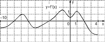
Let's get rid of unnecessary information. Let us leave only the boundaries [−10; 4] and zeros of the derivative, of which there were four this time: x = −8, x = −6, x = −3 and x = 2. Let’s mark the signs of the derivative and get the following picture:
We are interested in the intervals of increasing function, i.e. such where f’(x) ≥ 0. There are two such intervals on the graph: (−8; −6) and (−3; 2). Let's calculate their lengths:
l 1 = − 6 − (−8) = 2;
l 2 = 2 − (−3) = 5.
Since we need to find the length of the largest of the intervals, we write down the value l 2 = 5 as an answer.
The operation of finding the derivative is called differentiation.
As a result of solving problems of finding derivatives of the simplest (and not very simple) functions by defining the derivative as the limit of the ratio of the increment to the increment of the argument, a table of derivatives appeared and exactly certain rules differentiation. The first to work in the field of finding derivatives were Isaac Newton (1643-1727) and Gottfried Wilhelm Leibniz (1646-1716).
Therefore, in our time, to find the derivative of any function, you do not need to calculate the above-mentioned limit of the ratio of the increment of the function to the increment of the argument, but you only need to use the table of derivatives and the rules of differentiation. The following algorithm is suitable for finding the derivative.
To find the derivative, you need an expression under the prime sign break down simple functions into components and determine what actions (product, sum, quotient) these functions are related. Further derivatives elementary functions we find in the table of derivatives, and the formulas for the derivatives of the product, sum and quotient are in the rules of differentiation. The derivative table and differentiation rules are given after the first two examples.
Example 1. Find the derivative of a function
Solution. From the rules of differentiation we find out that the derivative of a sum of functions is the sum of derivatives of functions, i.e.
From the table of derivatives we find out that the derivative of "x" is equal to one, and the derivative of sine is equal to cosine. We substitute these values into the sum of derivatives and find the derivative required by the condition of the problem:
Example 2. Find the derivative of a function
Solution. We differentiate as a derivative of a sum in which the second term has a constant factor; it can be taken out of the sign of the derivative:
![]()
If questions still arise about where something comes from, they are usually cleared up after familiarizing yourself with the table of derivatives and the simplest rules of differentiation. We are moving on to them right now.
Table of derivatives of simple functions
| 1. Derivative of a constant (number). Any number (1, 2, 5, 200...) that is in the function expression. Always equal to zero. This is very important to remember, as it is required very often | |
| 2. Derivative of the independent variable. Most often "X". Always equal to one. This is also important to remember for a long time | |
| 3. Derivative of degree. When solving problems, you need to convert non-square roots into powers. | |
| 4. Derivative of a variable to the power -1 | |
| 5. Derivative square root | |
| 6. Derivative of sine | |
| 7. Derivative of cosine | |
| 8. Derivative of tangent | |
| 9. Derivative of cotangent | |
| 10. Derivative of arcsine | |
| 11. Derivative of arccosine | |
| 12. Derivative of arctangent | |
| 13. Derivative of arc cotangent | |
| 14. Derivative of the natural logarithm | |
| 15. Derivative of a logarithmic function | |
| 16. Derivative of the exponent | |
| 17. Derivative of an exponential function |
Rules of differentiation
| 1. Derivative of a sum or difference | |
| 2. Derivative of the product | |
| 2a. Derivative of an expression multiplied by a constant factor | |
| 3. Derivative of the quotient | |
| 4. Derivative of a complex function |  |
Rule 1.If the functions
are differentiable at some point, then the functions are differentiable at the same point
and
![]()
those. the derivative of the algebraic sum of functions is equal to algebraic sum derivatives of these functions.
Consequence. If two differentiable functions differ by a constant term, then their derivatives are equal, i.e.
Rule 2.If the functions
are differentiable at some point, then their product is differentiable at the same point
and
![]()
those. The derivative of the product of two functions is equal to the sum of the products of each of these functions and the derivative of the other.
Corollary 1. The constant factor can be taken out of the sign of the derivative:
Corollary 2. The derivative of the product of several differentiable functions is equal to the sum of the products of the derivative of each factor and all the others.
For example, for three multipliers:
Rule 3.If the functions
differentiable at some point And , then at this point their quotient is also differentiableu/v , and
![]()
those. the derivative of the quotient of two functions is equal to a fraction, the numerator of which is the difference between the products of the denominator and the derivative of the numerator and the numerator and the derivative of the denominator, and the denominator is the square of the former numerator.
Where to look for things on other pages
When finding the derivative of a product and the quotient in real problems It is always necessary to apply several differentiation rules at once, therefore more examples for these derivatives - in the article"Derivative of the product and quotient of functions".
Comment. You should not confuse a constant (that is, a number) as a term in a sum and as a constant factor! In the case of a term, its derivative is equal to zero, and in the case constant factor it is taken out of the derivative sign. This typical mistake, which occurs on initial stage studying derivatives, but as they solve several one- and two-part examples, the average student no longer makes this mistake.
And if, when differentiating a product or quotient, you have a term u"v, in which u- a number, for example, 2 or 5, that is, a constant, then the derivative of this number will be equal to zero and, therefore, the entire term will be equal to zero (this case is discussed in example 10).
Other common mistake - mechanical solution derivative of a complex function as a derivative of a simple function. That's why derivative of a complex function a separate article is devoted. But first we will learn to find derivatives simple functions.
Along the way, you can’t do without transforming expressions. To do this, you may need to open the manual in new windows. Actions with powers and roots And Operations with fractions .
If you are looking for solutions to derivatives of fractions with powers and roots, that is, when the function looks like ![]() , then follow the lesson “Derivative of sums of fractions with powers and roots.”
, then follow the lesson “Derivative of sums of fractions with powers and roots.”
If you have a task like ![]() , then you will take the lesson “Derivatives of simple trigonometric functions”.
, then you will take the lesson “Derivatives of simple trigonometric functions”.
Step-by-step examples - how to find the derivative
Example 3. Find the derivative of a function
Solution. We define the parts of the function expression: the entire expression represents a product, and its factors are sums, in the second of which one of the terms contains a constant factor. We apply the product differentiation rule: the derivative of the product of two functions is equal to the sum of the products of each of these functions by the derivative of the other:
![]()
Next, we apply the rule of differentiation of the sum: the derivative of the algebraic sum of functions is equal to the algebraic sum of the derivatives of these functions. In our case, in each sum the second term has a minus sign. In each sum we see both an independent variable, the derivative of which is equal to one, and a constant (number), the derivative of which is equal to zero. So, “X” turns into one, and minus 5 turns into zero. In the second expression, "x" is multiplied by 2, so we multiply two by the same unit as the derivative of "x". We obtain the following derivative values:
We substitute the found derivatives into the sum of products and obtain the derivative of the entire function required by the condition of the problem:
![]()
Example 4. Find the derivative of a function
Solution. We are required to find the derivative of the quotient. We apply the formula for differentiating the quotient: the derivative of the quotient of two functions is equal to a fraction, the numerator of which is the difference between the products of the denominator and the derivative of the numerator and the numerator and the derivative of the denominator, and the denominator is the square of the former numerator. We get:

We have already found the derivative of the factors in the numerator in example 2. Let us also not forget that the product, which is the second factor in the numerator in the current example, is taken with a minus sign:

If you are looking for solutions to problems in which you need to find the derivative of a function, where there is a continuous pile of roots and powers, such as, for example, ![]() , then welcome to class "Derivative of sums of fractions with powers and roots" .
, then welcome to class "Derivative of sums of fractions with powers and roots" .
If you need to learn more about the derivatives of sines, cosines, tangents and others trigonometric functions, that is, when the function looks like ![]() , then a lesson for you "Derivatives of simple trigonometric functions" .
, then a lesson for you "Derivatives of simple trigonometric functions" .
Example 5. Find the derivative of a function
Solution. In this function we see a product, one of the factors of which is the square root of the independent variable, the derivative of which we familiarized ourselves with in the table of derivatives. Using the rule for differentiating the product and the tabular value of the derivative of the square root, we obtain:

Example 6. Find the derivative of a function
Solution. In this function we see a quotient whose dividend is the square root of the independent variable. Using the rule of differentiation of quotients, which we repeated and applied in example 4, and the tabulated value of the derivative of the square root, we obtain:

To get rid of a fraction in the numerator, multiply the numerator and denominator by .
Continuity and differentiability of a function.
Darboux's theorem . Intervals of monotony.
Critical points . Extremum (minimum, maximum).
Function study design.
Relationship between continuity and differentiability of a function. If function f(x)is differentiable at some point, then it is continuous at that point. The reverse is not true: a continuous function may not have a derivative.
Illustration. If the function is discontinuous at some point, then it has no derivative at this point.

Sufficient signs of monotonicity of a function.
If f’(x) > 0 at each point of the interval (a, b), then the function f (x)increases over this interval.
If f’(x) < 0 at each point of the interval (a, b) , then the function f(x)decreases on this interval.
Darboux's theorem. Points at which the derivative of a function is 0or does not exist, divide the domain of definition of the function into intervals within which the derivative retains its sign.
Using these intervals we can find intervals of monotony functions, which is very important when studying them.


Consequently, the function increases over the intervals (- , 0) and ( 1, + ) and decreases on the interval ( 0, 1). Dot x= 0 is not included in the definition domain of the function, but as we get closerx k0 term x - 2 increases indefinitely, so the function also increases indefinitely. At the pointx= 1 the value of the function is 3. According to this analysis we can postgraph the function ( Fig.4 b ) .
Critical points. Interior points of the function domain, in which the derivative is equal to null or does not exist, are called critical dots this function. These points are very important when analyzing a function and plotting its graph, because only at these points can a function have extremum (minimum or maximum , Fig.5 A,b).

At points x 1 , x 2 (Fig.5 a) And x 3 (Fig.5 b) derivative is 0; at points x 1 , x 2 (Fig.5 b) derivative does not exist. But they are all extreme points.
A necessary condition for an extremum. If x 0 - extremum point of the function f(x) and the derivative f’ exists at this point, then f’(x 0)= 0.
This theorem is necessary extremum condition. If the derivative of a function at some point is 0, that doesn't mean that the function has an extremum at this point. For example, the derivative of the functionf (x) = x 3 equals 0 at x= 0, but this function does not have an extremum at this point (Fig. 6).

On the other hand, the functiony = | x| , presented in Fig. 3, has a minimum at the pointx= 0, but at this point the derivative does not exist.
Sufficient conditions for an extremum.
If the derivative when passing through the point x 0 changes its sign from plus to minus, then x 0 - maximum point.
If the derivative when passing through the point x 0 changes its sign from minus to plus, then x 0 - minimum point.
Function study design. To plot a function graph you need:
1) find the domain of definition and range of values of the function,
2) determine whether the function is even or odd,
3) determine whether the function is periodic or not,
4) find the zeros of the function and its values atx = 0,
5) find intervals of constant sign,
6) find intervals of monotonicity,
7) find extremum points and function values at these points,
8) analyze the behavior of the function near “singular” points
And when large values modulex .
EXAMPLE Explore the featuref(x) = x 3 + 2 x 2 - x- 2 and draw a graph.
Solution. Let's study the function according to the above diagram.
1) domainxR (x– any real number);
Range of valuesyR , because f (x) – odd polynomial
degrees;
2) function f (x) is neither even nor odd
(clarify please);
3) f (x) is a non-periodic function (prove it yourself);
4) the graph of the function intersects the axisY at point (0, – 2),
Because f (0) = - 2 ; to find the zeros of the function you need
Solve the equation:x 3 + 2 x 2 - x - 2 = 0, one of the roots
Which ( x= 1) is obvious. Other roots are
(if they are! ) from solving the quadratic equation:
x 2 + 3 x+ 2 = 0, which is obtained by dividing the polynomial
x 3 + 2 x 2 - x- 2 per binomial ( x- 1). Easy to check
What are the other two roots:x 2 = - 2 and x 3 = - 1. Thus,
The zeros of the function are: - 2, - 1 and 1.
5) This means that the number axis is divided by these roots by
Four intervals of constancy of sign, within which
The function retains its sign:
This result can be obtained by expanding
polynomial into factors:
x 3 + 2 x 2 - x - 2 = (x + 2) (x + 1 (x – 1)
And an assessment of the sign of the work .
6) Derivative f' (x) = 3 x 2 + 4 x- 1 has no points at which
It does not exist, so its domain of definition isR (All
Real numbers); zerosf' (x) are the roots of the equation:
3 x 2 + 4 x- 1 = 0 .

The results obtained are summarized in the table:

When deciding various tasks geometry, mechanics, physics and other branches of knowledge became necessary using the same analytical process from this function y=f(x) receive new feature which is called derivative function(or simply derivative) of a given function f(x) and is designated by the symbol
The process by which from a given function f(x) get a new feature f" (x), called differentiation and it consists of the following three steps: 1) give the argument x increment
x and determine the corresponding increment of the function
y = f(x+
x) -f(x); 2) make up a relation 
3) counting x constant and
x0, we find  , which we denote by f" (x), as if emphasizing that the resulting function depends only on the value x, at which we go to the limit. Definition:
Derivative y " =f " (x)
given function y=f(x)
for a given x is called the limit of the ratio of the increment of a function to the increment of the argument, provided that the increment of the argument tends to zero, if, of course, this limit exists, i.e. finite. Thus,
, which we denote by f" (x), as if emphasizing that the resulting function depends only on the value x, at which we go to the limit. Definition:
Derivative y " =f " (x)
given function y=f(x)
for a given x is called the limit of the ratio of the increment of a function to the increment of the argument, provided that the increment of the argument tends to zero, if, of course, this limit exists, i.e. finite. Thus,  , or
, or 
Note that if for some value x, for example when x=a, attitude  at
x0 does not tend to finite limit, then in this case they say that the function f(x) at x=a(or at the point x=a) has no derivative or is not differentiable at the point x=a.
at
x0 does not tend to finite limit, then in this case they say that the function f(x) at x=a(or at the point x=a) has no derivative or is not differentiable at the point x=a.
2. Geometric meaning of the derivative.
Consider the graph of the function y = f (x), differentiable in the vicinity of the point x 0

f(x)
Let's consider an arbitrary straight line passing through a point on the graph of a function - point A(x 0 , f (x 0)) and intersecting the graph at some point B(x;f(x)). Such a line (AB) is called a secant. From ∆ABC: AC = ∆x; BC =∆у; tgβ=∆y/∆x.
Since AC || Ox, then ALO = BAC = β (as corresponding for parallel). But ALO is the angle of inclination of the secant AB to the positive direction of the Ox axis. This means that tanβ = k is the slope of straight line AB.
Now we will reduce ∆х, i.e. ∆х→ 0. In this case, point B will approach point A according to the graph, and secant AB will rotate. The limiting position of the secant AB at ∆x→ 0 will be a straight line (a), called the tangent to the graph of the function y = f (x) at point A.
If we go to the limit as ∆x → 0 in the equality tgβ =∆y/∆x, we get  ortg =f "(x 0), since
  -angle of inclination of the tangent to the positive direction of the Ox axis
  , by definition of a derivative. But tg = k is the angular coefficient of the tangent, which means k = tg = f "(x 0).
So, the geometric meaning of the derivative is as follows:
Derivative of a function at point x 0 equal to the slope of the tangent to the graph of the function drawn at the point with the abscissa x 0 .
3. Physical meaning of the derivative.
Consider the movement of a point along a straight line. Let the coordinate of a point at any time x(t) be given. It is known (from a physics course) that the average speed over a period of time is equal to the ratio of the distance traveled during this period of time to the time, i.e.
Vav = ∆x/∆t. Let's go to the limit in the last equality as ∆t → 0.
lim Vav (t) = (t 0) - instantaneous speed at time t 0, ∆t → 0.
and lim = ∆x/∆t = x"(t 0) (by definition of derivative).
So, (t) =x"(t).
The physical meaning of the derivative is as follows: derivative of the functiony = f(x) at pointx 0 is the rate of change of the functionf(x) at pointx 0
The derivative is used in physics to find velocity from a known function of coordinates versus time, acceleration from a known function of velocity versus time.
(t) = x"(t) - speed,
a(f) = "(t) - acceleration, or
If the law of motion of a material point in a circle is known, then one can find the angular velocity and angular acceleration during rotational movement:
φ = φ(t) - change in angle over time,
ω = φ"(t) - angular velocity,
ε = φ"(t) - angular acceleration, or ε = φ"(t).
If the law of mass distribution of an inhomogeneous rod is known, then the linear density of the inhomogeneous rod can be found:
m = m(x) - mass,
x , l - length of the rod,
p = m"(x) - linear density.
Using the derivative, problems from the theory of elasticity and harmonic vibrations are solved. So, according to Hooke's law
F = -kx, x – variable coordinate, k – spring elasticity coefficient. Putting ω 2 =k/m, we obtain the differential equation of the spring pendulum x"(t) + ω 2 x(t) = 0,
where ω = √k/√m oscillation frequency (l/c), k - spring stiffness (H/m).
An equation of the form y" + ω 2 y = 0 is called the equation of harmonic oscillations (mechanical, electrical, electromagnetic). The solution to such equations is the function
y = Asin(ωt + φ 0) or y = Acos(ωt + φ 0), where
A - amplitude of oscillations, ω - cyclic frequency,
φ 0 - initial phase.