Examples of systems of linear equations: solution method. Simple and complex methods for solving systems of equations

I. Ordinary differential equations

1.1. Basic concepts and definitions

A differential equation is an equation that relates an independent variable x, the required function y and its derivatives or differentials.

Symbolically, the differential equation is written as follows:

F(x,y,y")=0, F(x,y,y")=0, F(x,y,y",y",.., y (n))=0

A differential equation is called ordinary if the required function depends on one independent variable.

Solving a differential equation is called a function that turns this equation into an identity.

The order of the differential equation is the order of the highest derivative included in this equation

Examples.

1. Consider a first order differential equation

The solution to this equation is the function y = 5 ln x. Indeed, substituting y" into the equation, we get the identity.

And this means that the function y = 5 ln x– is a solution to this differential equation.

2. Consider the second order differential equation y" - 5y" +6y = 0. The function is the solution to this equation.

Really, .

Substituting these expressions into the equation, we obtain: , – identity.

And this means that the function is the solution to this differential equation.

Integrating differential equations is the process of finding solutions to differential equations.

General solution of the differential equation called a function of the form , which includes as many independent arbitrary constants as the order of the equation.

Partial solution of the differential equation is a solution obtained from a general solution for various numerical values of arbitrary constants. The values of arbitrary constants are found at certain initial values of the argument and function.

The graph of a particular solution to a differential equation is called integral curve.

Examples

1. Find a particular solution to a first order differential equation

xdx + ydy = 0, If y= 4 at x = 3.

Solution. Integrating both sides of the equation, we get

Comment. An arbitrary constant C obtained as a result of integration can be represented in any form convenient for further transformations. In this case, taking into account the canonical equation of a circle, it is convenient to represent an arbitrary constant C in the form .

- general solution of the differential equation.

Particular solution of the equation satisfying the initial conditions y = 4 at x = 3 is found from the general by substituting the initial conditions into the general solution: 3 2 + 4 2 = C 2 ; C=5.

Substituting C=5 into the general solution, we get x 2 +y 2 = 5 2 .

This is a particular solution to a differential equation obtained from a general solution under given initial conditions.

2. Find the general solution to the differential equation

The solution to this equation is any function of the form , where C is an arbitrary constant. Indeed, substituting into the equations, we obtain: , .

Consequently, this differential equation has an infinite number of solutions, since for different values of the constant C, equality determines different solutions to the equation.

For example, by direct substitution you can verify that the functions are solutions to the equation.

A problem in which you need to find a particular solution to the equation y" = f(x,y) satisfying the initial condition y(x 0) = y 0, is called the Cauchy problem.

Solving the equation y" = f(x,y), satisfying the initial condition, y(x 0) = y 0, is called a solution to the Cauchy problem.

The solution to the Cauchy problem has a simple geometric meaning. Indeed, according to these definitions, to solve the Cauchy problem y" = f(x,y) given that y(x 0) = y 0, means to find the integral curve of the equation y" = f(x,y) which passes through a given point M 0 (x 0,y 0).

II. First order differential equations

2.1. Basic Concepts

A first order differential equation is an equation of the form F(x,y,y") = 0.

A first order differential equation includes the first derivative and does not include higher order derivatives.

The equation y" = f(x,y) is called a first-order equation solved with respect to the derivative.

The general solution of a first-order differential equation is a function of the form , which contains one arbitrary constant.

Example. Consider a first order differential equation.

The solution to this equation is the function.

Indeed, replacing this equation with its value, we get

that is 3x=3x

Therefore, the function is a general solution to the equation for any constant C.

Find a particular solution to this equation that satisfies the initial condition y(1)=1 Substituting initial conditions x = 1, y =1 into the general solution of the equation, we get from where C=0.

Thus, we obtain a particular solution from the general one by substituting into this equation the resulting value C=0– private solution.

2.2. Differential equations with separable variables

A differential equation with separable variables is an equation of the form: y"=f(x)g(y) or through differentials, where f(x) And g(y)– specified functions.

For those y, for which , the equation y"=f(x)g(y) is equivalent to the equation, in which the variable y is present only on the left side, and the variable x is only on the right side. They say, "in Eq. y"=f(x)g(y Let's separate the variables."

Equation of the form called a separated variable equation.

Integrating both sides of the equation By x, we get G(y) = F(x) + C is the general solution of the equation, where G(y) And F(x)– some antiderivatives, respectively, of functions and f(x), C arbitrary constant.

Algorithm for solving a first order differential equation with separable variables

Example 1

Solve the equation y" = xy

Solution. Derivative of a function y" replace it with

let's separate the variables

Let's integrate both sides of the equality:

Example 2

2yy" = 1- 3x 2, If y 0 = 3 at x 0 = 1

This is a separated variable equation. Let's imagine it in differentials. To do this, we rewrite this equation in the form From here

Integrating both sides of the last equality, we find

Substituting the initial values x 0 = 1, y 0 = 3 we'll find WITH 9=1-1+C, i.e. C = 9.

Therefore, the required partial integral will be or

Example 3

Write an equation for a curve passing through a point M(2;-3) and having a tangent with an angular coefficient

Solution. According to the condition

This is an equation with separable variables. Dividing the variables, we get:

Integrating both sides of the equation, we get:

Using the initial conditions, x = 2 And y = - 3 we'll find C:

Therefore, the required equation has the form

2.3. Linear differential equations of the first order

A linear differential equation of the first order is an equation of the form y" = f(x)y + g(x)

Where f(x) And g(x)- some specified functions.

If g(x)=0 then the linear differential equation is called homogeneous and has the form: y" = f(x)y

If then the equation y" = f(x)y + g(x) is called heterogeneous.

General solution of a linear homogeneous differential equation y" = f(x)y is given by the formula: where WITH– arbitrary constant.

In particular, if C =0, then the solution is y = 0 If a linear homogeneous equation has the form y" = ky Where k is some constant, then its general solution has the form: .

General solution of a linear inhomogeneous differential equation y" = f(x)y + g(x) is given by the formula ,

those. is equal to the sum of the general solution of the corresponding linear homogeneous equation and the particular solution of this equation.

For a linear inhomogeneous equation of the form y" = kx + b,

Where k And b- some numbers and a particular solution will be a constant function. Therefore, the general solution has the form .

Example. Solve the equation y" + 2y +3 = 0

Solution. Let's represent the equation in the form y" = -2y - 3 Where k = -2, b= -3 The general solution is given by the formula.

Therefore, where C is an arbitrary constant.

2.4. Solving linear differential equations of the first order by the Bernoulli method

Finding a General Solution to a First Order Linear Differential Equation y" = f(x)y + g(x) reduces to solving two differential equations with separated variables using substitution y=uv, Where u And v- unknown functions from x. This solution method is called Bernoulli's method.

Algorithm for solving a first order linear differential equation

y" = f(x)y + g(x)

1. Enter substitution y=uv.

2. Differentiate this equality y" = u"v + uv"

3. Substitute y And y" into this equation: u"v + uv" =f(x)uv + g(x) or u"v + uv" + f(x)uv = g(x).

4. Group the terms of the equation so that u take it out of brackets:

5. From the bracket, equating it to zero, find the function

This is a separable equation:

Let's divide the variables and get:

Where . .

6. Substitute the resulting value v into the equation (from step 4):

and find the function This is an equation with separable variables:

7. Write the general solution in the form: , i.e. .

Example 1

Find a particular solution to the equation y" = -2y +3 = 0 If y =1 at x = 0

Solution. Let's solve it using substitution y=uv,.y" = u"v + uv"

Substituting y And y" into this equation, we get

By grouping the second and third terms on the left side of the equation, we take out the common factor u out of brackets

We equate the expression in brackets to zero and, having solved the resulting equation, we find the function v = v(x)

We get an equation with separated variables. Let's integrate both sides of this equation: Find the function v:

Let's substitute the resulting value v into the equation we get:

This is a separated variable equation. Let's integrate both sides of the equation: Let's find the function u = u(x,c) Let's find a general solution: Let us find a particular solution to the equation that satisfies the initial conditions y = 1 at x = 0:

III. Higher order differential equations

3.1. Basic concepts and definitions

A second-order differential equation is an equation containing derivatives of no higher than second order. In the general case, a second-order differential equation is written as: F(x,y,y",y") = 0

The general solution of a second-order differential equation is a function of the form , which includes two arbitrary constants C 1 And C 2.

A particular solution to a second-order differential equation is a solution obtained from a general solution for certain values of arbitrary constants C 1 And C 2.

3.2. Linear homogeneous differential equations of the second order with constant coefficients.

Linear homogeneous differential equation of the second order with constant coefficients called an equation of the form y" + py" +qy = 0, Where p And q- constant values.

Algorithm for solving homogeneous second order differential equations with constant coefficients

1. Write the differential equation in the form: y" + py" +qy = 0.

2. Create its characteristic equation, denoting y" through r 2, y" through r, y in 1: r 2 + pr +q = 0

1. Substitution method: from any equation of the system we express one unknown through another and substitute it into the second equation of the system.

Task. Solve the system of equations:

Solution. From the first equation of the system we express at through X and substitute it into the second equation of the system. Let's get the system equivalent to the original one.

After bringing similar terms, the system will take the form:

From the second equation we find: . Substituting this value into the equation at = 2 - 2X, we get at= 3. Therefore, the solution to this system is a pair of numbers.

2. Algebraic addition method: By adding two equations, you get an equation with one variable.

Task. Solve the system equation:

Solution. Multiplying both sides of the second equation by 2, we get the system equivalent to the original one. Adding the two equations of this system, we arrive at the system

After bringing similar terms, this system will take the form: From the second equation we find . Substituting this value into equation 3 X + 4at= 5, we get , where . Therefore, the solution to this system is a pair of numbers.

3. Method for introducing new variables: we are looking for some repeating expressions in the system, which we will denote by new variables, thereby simplifying the appearance of the system.

Task. Solve the system of equations:

Solution. Let's write this system differently:

Let x + y = u, xy = v. Then we get the system

Let's solve it using the substitution method. From the first equation of the system we express u through v and substitute it into the second equation of the system. Let's get the system those.

From the second equation of the system we find v 1 = 2, v 2 = 3.

Substituting these values into the equation u = 5 - v, we get u 1 = 3,
u 2 = 2. Then we have two systems

Solving the first system, we get two pairs of numbers (1; 2), (2; 1). The second system has no solutions.

Exercises for independent work

1. Solve systems of equations using the substitution method.

Systems of equations are widely used in the economic sector for mathematical modeling of various processes. For example, when solving problems of production management and planning, logistics routes (transport problem) or equipment placement.

Systems of equations are used not only in mathematics, but also in physics, chemistry and biology, when solving problems of finding population size.

A system of linear equations is two or more equations with several variables for which it is necessary to find a common solution. Such a sequence of numbers for which all equations become true equalities or prove that the sequence does not exist.

Linear equation

Equations of the form ax+by=c are called linear. The designations x, y are the unknowns whose value must be found, b, a are the coefficients of the variables, c is the free term of the equation.
Solving an equation by plotting it will look like a straight line, all points of which are solutions to the polynomial.

Types of systems of linear equations

The simplest examples are considered to be systems of linear equations with two variables X and Y.

F1(x, y) = 0 and F2(x, y) = 0, where F1,2 are functions and (x, y) are function variables.

Solve system of equations - this means finding values (x, y) at which the system turns into a true equality or establishing that suitable values of x and y do not exist.

A pair of values (x, y), written as the coordinates of a point, is called a solution to a system of linear equations.

If systems have one common solution or no solution exists, they are called equivalent.

Homogeneous systems of linear equations are systems whose right-hand side is equal to zero. If the right part after the equal sign has a value or is expressed by a function, such a system is heterogeneous.

The number of variables can be much more than two, then we should talk about an example of a system of linear equations with three or more variables.

When faced with systems, schoolchildren assume that the number of equations must necessarily coincide with the number of unknowns, but this is not the case. The number of equations in the system does not depend on the variables; there can be as many of them as desired.

Simple and complex methods for solving systems of equations

There is no general analytical method for solving such systems; all methods are based on numerical solutions. The school mathematics course describes in detail such methods as permutation, algebraic addition, substitution, as well as graphical and matrix methods, solution by the Gaussian method.

The main task when teaching solution methods is to teach how to correctly analyze the system and find the optimal solution algorithm for each example. The main thing is not to memorize a system of rules and actions for each method, but to understand the principles of using a particular method

Solving examples of systems of linear equations in the 7th grade general education curriculum is quite simple and explained in great detail. In any mathematics textbook, this section is given enough attention. Solving examples of systems of linear equations using the Gauss and Cramer method is studied in more detail in the first years of higher education.

Solving systems using the substitution method

The actions of the substitution method are aimed at expressing the value of one variable in terms of the second. The expression is substituted into the remaining equation, then it is reduced to a form with one variable. The action is repeated depending on the number of unknowns in the system

Let us give a solution to an example of a system of linear equations of class 7 using the substitution method:

As can be seen from the example, the variable x was expressed through F(X) = 7 + Y. The resulting expression, substituted into the 2nd equation of the system in place of X, helped to obtain one variable Y in the 2nd equation. Solving this example is easy and allows you to get the Y value. The last step is to check the obtained values.

It is not always possible to solve an example of a system of linear equations by substitution. The equations can be complex and expressing the variable in terms of the second unknown will be too cumbersome for further calculations. When there are more than 3 unknowns in the system, solving by substitution is also inappropriate.

Solution of an example of a system of linear inhomogeneous equations:

Solution using algebraic addition

When searching for solutions to systems using the addition method, equations are added term by term and multiplied by various numbers. The ultimate goal of mathematical operations is an equation in one variable.

Application of this method requires practice and observation. Solving a system of linear equations using the addition method when there are 3 or more variables is not easy. Algebraic addition is convenient to use when equations contain fractions and decimals.

Solution algorithm:

Multiply both sides of the equation by a certain number. As a result of the arithmetic operation, one of the coefficients of the variable should become equal to 1.
Add the resulting expression term by term and find one of the unknowns.
Substitute the resulting value into the 2nd equation of the system to find the remaining variable.

Method of solution by introducing a new variable

A new variable can be introduced if the system requires finding a solution for no more than two equations; the number of unknowns should also be no more than two.

The method is used to simplify one of the equations by introducing a new variable. The new equation is solved for the introduced unknown, and the resulting value is used to determine the original variable.

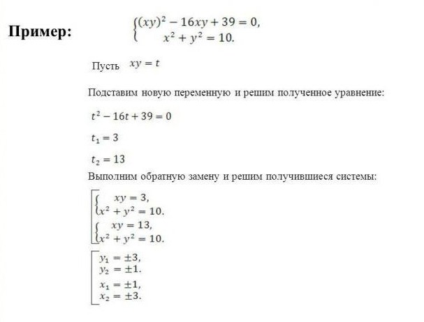
The example shows that by introducing a new variable t, it was possible to reduce the 1st equation of the system to a standard quadratic trinomial. You can solve a polynomial by finding the discriminant.

It is necessary to find the value of the discriminant using the well-known formula: D = b2 - 4*a*c, where D is the desired discriminant, b, a, c are the factors of the polynomial. In the given example, a=1, b=16, c=39, therefore D=100. If the discriminant is greater than zero, then there are two solutions: t = -b±√D / 2*a, if the discriminant is less than zero, then there is one solution: x = -b / 2*a.

The solution for the resulting systems is found by the addition method.

Visual method for solving systems

Suitable for 3 equation systems. The method consists in constructing graphs of each equation included in the system on the coordinate axis. The coordinates of the intersection points of the curves will be the general solution of the system.

The graphical method has a number of nuances. Let's look at several examples of solving systems of linear equations in a visual way.

As can be seen from the example, for each line two points were constructed, the values of the variable x were chosen arbitrarily: 0 and 3. Based on the values of x, the values for y were found: 3 and 0. Points with coordinates (0, 3) and (3, 0) were marked on the graph and connected by a line.

The steps must be repeated for the second equation. The point of intersection of the lines is the solution of the system.

The following example requires finding a graphical solution to a system of linear equations: 0.5x-y+2=0 and 0.5x-y-1=0.

As can be seen from the example, the system has no solution, because the graphs are parallel and do not intersect along their entire length.

The systems from examples 2 and 3 are similar, but when constructed it becomes obvious that their solutions are different. It should be remembered that it is not always possible to say whether a system has a solution or not; it is always necessary to construct a graph.

The matrix and its varieties

Matrices are used to concisely write a system of linear equations. A matrix is a special type of table filled with numbers. n*m has n - rows and m - columns.

A matrix is square when the number of columns and rows are equal. A matrix-vector is a matrix of one column with an infinitely possible number of rows. A matrix with ones along one of the diagonals and other zero elements is called identity.

An inverse matrix is a matrix when multiplied by which the original one turns into a unit matrix; such a matrix exists only for the original square one.

Rules for converting a system of equations into a matrix

In relation to systems of equations, the coefficients and free terms of the equations are written as matrix numbers; one equation is one row of the matrix.

A matrix row is said to be nonzero if at least one element of the row is not zero. Therefore, if in any of the equations the number of variables differs, then it is necessary to enter zero in place of the missing unknown.

The matrix columns must strictly correspond to the variables. This means that the coefficients of the variable x can be written only in one column, for example the first, the coefficient of the unknown y - only in the second.

When multiplying a matrix, all elements of the matrix are sequentially multiplied by a number.

Options for finding the inverse matrix

The formula for finding the inverse matrix is quite simple: K -1 = 1 / |K|, where K -1 is the inverse matrix, and |K| is the determinant of the matrix. |K| must not be equal to zero, then the system has a solution.

The determinant is easily calculated for a two-by-two matrix; you just need to multiply the diagonal elements by each other. For the “three by three” option, there is a formula |K|=a 1 b 2 c 3 + a 1 b 3 c 2 + a 3 b 1 c 2 + a 2 b 3 c 1 + a 2 b 1 c 3 + a 3 b 2 c 1 . You can use the formula, or you can remember that you need to take one element from each row and each column so that the numbers of columns and rows of elements are not repeated in the work.

Solving examples of systems of linear equations using the matrix method

The matrix method of finding a solution allows you to reduce cumbersome entries when solving systems with a large number of variables and equations.

In the example, a nm are the coefficients of the equations, the matrix is a vector x n are variables, and b n are free terms.

Solving systems using the Gaussian method

In higher mathematics, the Gaussian method is studied together with the Cramer method, and the process of finding solutions to systems is called the Gauss-Cramer solution method. These methods are used to find variables of systems with a large number of linear equations.

The Gauss method is very similar to solutions by substitution and algebraic addition, but is more systematic. In the school course, the solution by the Gaussian method is used for systems of 3 and 4 equations. The purpose of the method is to reduce the system to the form of an inverted trapezoid. By means of algebraic transformations and substitutions, the value of one variable is found in one of the equations of the system. The second equation is an expression with 2 unknowns, while 3 and 4 are, respectively, with 3 and 4 variables.

After bringing the system to the described form, the further solution is reduced to the sequential substitution of known variables into the equations of the system.

In school textbooks for grade 7, an example of a solution by the Gauss method is described as follows:

As can be seen from the example, at step (3) two equations were obtained: 3x 3 -2x 4 =11 and 3x 3 +2x 4 =7. Solving any of the equations will allow you to find out one of the variables x n.

Theorem 5, which is mentioned in the text, states that if one of the equations of the system is replaced by an equivalent one, then the resulting system will also be equivalent to the original one.

The Gaussian method is difficult for middle school students to understand, but it is one of the most interesting ways to develop the ingenuity of children enrolled in advanced learning programs in math and physics classes.

For ease of recording, calculations are usually done as follows:

The coefficients of the equations and free terms are written in the form of a matrix, where each row of the matrix corresponds to one of the equations of the system. separates the left side of the equation from the right. Roman numerals indicate the numbers of equations in the system.

First, write down the matrix to be worked with, then all the actions carried out with one of the rows. The resulting matrix is written after the "arrow" sign and the necessary algebraic operations are continued until the result is achieved.

The result should be a matrix in which one of the diagonals is equal to 1, and all other coefficients are equal to zero, that is, the matrix is reduced to a unit form. We must not forget to perform calculations with numbers on both sides of the equation.

This recording method is less cumbersome and allows you not to be distracted by listing numerous unknowns.

The free use of any solution method will require care and some experience. Not all methods are of an applied nature. Some methods of finding solutions are more preferable in a particular area of human activity, while others exist for educational purposes.

Maintaining your privacy is important to us. For this reason, we have developed a Privacy Policy that describes how we use and store your information. Please review our privacy practices and let us know if you have any questions.

Collection and use of personal information

Personal information refers to data that can be used to identify or contact a specific person.

You may be asked to provide your personal information at any time when you contact us.

Below are some examples of the types of personal information we may collect and how we may use such information.

What personal information do we collect:

When you submit an application on the site, we may collect various information, including your name, telephone number, email address, etc.

How we use your personal information:

The personal information we collect allows us to contact you with unique offers, promotions and other events and upcoming events.
From time to time, we may use your personal information to send important notices and communications.
We may also use personal information for internal purposes, such as conducting audits, data analysis and various research in order to improve the services we provide and provide you with recommendations regarding our services.
If you participate in a prize draw, contest or similar promotion, we may use the information you provide to administer such programs.

Disclosure of information to third parties

We do not disclose the information received from you to third parties.

Exceptions:

If necessary - in accordance with the law, judicial procedure, in legal proceedings, and/or on the basis of public requests or requests from government authorities in the territory of the Russian Federation - to disclose your personal information. We may also disclose information about you if we determine that such disclosure is necessary or appropriate for security, law enforcement, or other public importance purposes.
In the event of a reorganization, merger, or sale, we may transfer the personal information we collect to the applicable successor third party.

Protection of personal information

We take precautions - including administrative, technical and physical - to protect your personal information from loss, theft, and misuse, as well as unauthorized access, disclosure, alteration and destruction.

Respecting your privacy at the company level

To ensure that your personal information is secure, we communicate privacy and security standards to our employees and strictly enforce privacy practices.

Equations and systems of equations of the first degree

Two numbers or any expressions connected by the “=” sign form equality. If given numbers or expressions are equal for any values of the letters, then such equality is called identity.

For example, when they claim that for any A valid:

A + 1 = 1 + A, here equality is identity.

Equation is called an equality containing unknown numbers indicated by letters. These letters are called unknown. There may be several unknowns in the equation.

For example, in equation 2 X + at = 7X– 3 two unknowns: X And at.

The expression on the left in the equation (2 X + at) is called the left side of the equation, and the expression on the right side of the equation (7 X– 3), is called its right side.

The value of the unknown at which the equation becomes an identity is called decision or root equations

For example, if in equation 3 X+ 7=13 instead of unknown X substitute the number 2, we get the identity . Therefore, the value X= 2 satisfies the given equation and the number 2 is the solution or root of the given equation.

The two equations are called equivalent(or equivalent), if all solutions to the first equation are solutions to the second and vice versa, all solutions to the second equation are solutions to the first. Equivalent equations also include equations that have no solutions.

For example, equations 2 X– 5 = 11 and 7 X+ 6 = 62 are equivalent since they have the same root X= 8; equations X + 2 = X+ 5 and 2 X + 7 = 2X are equivalent because both have no solutions.

Properties of equivalent equations

1. To both sides of the equation you can add any expression that makes sense for all permissible values of the unknown; the resulting equation will be equivalent to the given one.

Example. Equation 2 X– 1 = 7 has a root X= 4. Adding 5 to both sides, we get equation 2 X– 1 + 5 = 7 + 5 or 2 X+ 4 = 12, which has the same root X = 4.

2. If both sides of the equation have identical terms, then they can be omitted.

Example. Equation 9 x + 5X = 18 + 5X has one root X= 2. Omitting 5 in both parts X, we get equation 9 X= 18, which has the same root X = 2.

3. Any member of the equation can be transferred from one part of the equation to another by changing its sign to the opposite.

Example. Equation 7 X - 11 = 3 has one root X= 2. If we move 11 to the right side with the opposite sign, we get equation 7 X= 3 + 11, which has the same solution X = 2.

4. Both sides of the equation can be multiplied by any expression (number) that makes sense and is different from zero for all acceptable values of the unknown, the resulting equation will be equivalent to the given one.

Example. Equation 2 X - 15 = 10 – 3X has a root X= 5. Multiplying both sides by 3, we get the equation 3(2 X - 15) = 3(10 – 3X) or 6 X – 45 =30 – 9X, which has the same root X = 5.

5. The signs of all terms of the equation can be reversed (this is equivalent to multiplying both sides by (-1)).

Example. Equation – 3 x + 7 = – 8 after multiplying both sides by (-1) will take the form 3 X - 7 = 8. The first and second equations have a single root X = 5.

6. Both sides of the equation can be divided by the same number that is different from zero (that is, not equal to zero).

Example..gif" width="49 height=25" height="25">.gif" width="131" height="28">, equivalent to this one, since it has the same two roots: and https:/ /pandia.ru/text/78/105/images/image006_96.gif" width="125" height="48 src="> after multiplying both parts by 14 it will look like:

https://pandia.ru/text/78/105/images/image009_71.gif" width="77 height=20" height="20">, where are arbitrary numbers, X- the unknown is called equation of the first degree with one unknown(or linear equation with one unknown).

Example. 2 X + 3 = 7 – 0,5X ; 0,3X = 0.

A first degree equation with one unknown always has one solution; a linear equation may have no solutions () or have an infinite number of them (https://pandia.ru/text/78/105/images/image013_59.gif" width="344 height=48" height="48">.

Solution. Multiply all terms in the equation by the least common multiple of the denominators, which is 12.

https://pandia.ru/text/78/105/images/image015_49.gif" width="183 height=24" height="24">.gif" width="371" height="20 src="> .

Let us group in one part (left) the terms containing the unknown, and in the other part (right) - free terms:

https://pandia.ru/text/78/105/images/image019_34.gif" width="104" height="20">. Dividing both parts by (-22), we get X = 7.

Systems of two equations of the first degree with two unknowns

An equation of the form https://pandia.ru/text/78/105/images/image021_34.gif" width="87" height="24 src="> is called equation of the first degree with two unknowns x And at. If general solutions to two or more equations are found, then they say that these equations form a system; they are usually written one under the other and combined with a curly brace, for example.

Each pair of unknown values that simultaneously satisfies both equations of the system is called system solution. Solve the system- this means finding all the solutions to this system or showing that it does not have them. The two systems of equations are called equivalent (equivalent), if all solutions of one of them are solutions of the other and vice versa, all solutions of the other are solutions of the first.

For example, the solution to the system is a pair of numbers X= 4 and at= 3. These numbers are also the only solution to the system . Therefore, these systems of equations are equivalent.

Methods for solving systems of equations

1. Method of algebraic addition. If the coefficients for some unknown in both equations are equal in absolute value, then by adding both equations (or subtracting one from the other), you can obtain an equation with one unknown. By solving this equation, one unknown is determined, and by substituting it into one of the equations of the system, the second unknown is found.

Examples: Solve systems of equations: 1) .

Here the coefficients for at are equal in absolute value, but opposite in sign. To obtain an equation with one unknown, we add the equations of the system term by term:

Received value X= 4 we substitute into some equation of the system, for example into the first one, and find the value at: .

Answer: X = 4; at = 3.

2) https://pandia.ru/text/78/105/images/image029_23.gif" width="112" height="57 src=">.gif" width="220" height="87 src=" >

https://pandia.ru/text/78/105/images/image033_21.gif" width="103" height="47 src=">.

2. Substitution method. From any equation of the system, we express one of the unknowns through the others, and then substitute the value of this unknown into the remaining equations. Let's look at this method using specific examples:

1) Let's solve the system of equations. Let us express one of the unknowns from the first equation, for example X: https://pandia.ru/text/78/105/images/image036_18.gif" width="483" height="24 src=">

Let's substitute at= 1 in the expression for X, we get .

Answer: https://pandia.ru/text/78/105/images/image039_18.gif" width="99" height="55 src=">. In this case, it is convenient to express at from the second equation:

https://pandia.ru/text/78/105/images/image041_16.gif" width="660" height="24">Substitute the value X= 5 in the expression for at, we get https://pandia.ru/text/78/105/images/image043_15.gif" width="96" height="24 src=">.

3) Let’s solve the system of equations https://pandia.ru/text/78/105/images/image045_12.gif" width="205" height="48">. Substituting this value into the second equation, we get an equation with one unknown at: https://pandia.ru/text/78/105/images/image049_11.gif" width="128" height="48">

Answer: https://pandia.ru/text/78/105/images/image051_12.gif" width="95" height="108 src="> .

Let's rewrite the system in the form: . We replace the unknowns by putting , and we obtain a linear system ..gif" width="11 height=17" height="17"> into the second equation, we get an equation with one unknown:

Substituting the value v into an expression for t, we get: https://pandia.ru/text/78/105/images/image060_9.gif" width="92 height=51" height="51"> we find.

Answer: https://pandia.ru/text/78/105/images/image062_9.gif" width="120" height="57">, where are the coefficients for unknowns, https://pandia.ru/text/ 78/105/images/image065_10.gif" width="67" height="52 src=">, then the system has the only thing solution.

B) If https://pandia.ru/text/78/105/images/image067_9.gif" width="105" height="52 src=">, then the system has infinite set decisions.

Example..gif" width="47" height="48 src=">", which means the system has a unique solution.

Really, .

https://pandia.ru/text/78/105/images/image073_7.gif" width="115" height="48 src=">.

Example..gif" width="91 height=48" height="48"> or after reduction, therefore, the system has no solutions.

Example..gif" width="116 height=48" height="48"> or after reduction , which means the system has an infinite number of solutions.

Equations containing modulus

When solving equations containing a modulus, the concept of the modulus of a real number is used. Module (absolute value) real number A this number itself is called if the opposite number (– A), if https://pandia.ru/text/78/105/images/image082_7.gif" width="20" height="28">.

So, https://pandia.ru/text/78/105/images/image084_8.gif" width="44" height="28 src=">, since the number 3 > 0; since the number is 5< 0, поэтому ; , because (); , because .

Module properties:

1) https://pandia.ru/text/78/105/images/image093_7.gif" width="72" height="28 src=">

3) https://pandia.ru/text/78/105/images/image095_8.gif" width="123" height="56 src=">

5) https://pandia.ru/text/78/105/images/image097_7.gif" width="73" height="28 src=">.

Considering that the expression under the module can take two values https://pandia.ru/text/78/105/images/image099_8.gif" width="68" height="20 src=">, then this equation comes down to solving two equations: and or And ..gif" width="52" height="20 src=">. Let's check by substituting each value X in the condition: if https://pandia.ru/text/78/105/images/image106_5.gif" width="165" height="28 src=">..gif" width="144" height="28 src=">.

Answer: https://pandia.ru/text/78/105/images/image104_6.gif" width="49" height="20 src=">.

Example..gif" width="408" height="55">

Answer: https://pandia.ru/text/78/105/images/image111_6.gif" width="41" height="20 src=">.

Example..gif" width="137" height="20"> and . Set aside the received values X on the number line, dividing it into intervals:

If https://pandia.ru/text/78/105/images/image117_5.gif" width="144" height="24">, because in this interval, both expressions under the modulus sign are less than zero, and , removing the module, we must change the sign of the expression to the opposite. Solve the resulting equation:

Gif" width="75 height=24" height="24">. The boundary value can be included in both the first and second interval, just as the value can be included in both the second and third. In the second interval, our equation will take the form: - this expression does not make sense, i.e. on this interval the equation has no solutions under the modulus sign, we equate them to zero. We find the roots of all expressions, with

Next interval https://pandia.ru/text/78/105/images/image124_6.gif" width="225" height="20">..gif" width="52" height="20 src="> .gif" width="125" height="25">, where a, b, c– arbitrary numbers ( a≠ 0), and x- a variable called square. To solve such an equation, you need to calculate the discriminant D=b 2 – 4ac. If D> 0, then the quadratic equation has two solutions (roots): And .

If D= 0, the quadratic equation obviously has two identical solutions (multiples of the root).

If D< 0, квадратное уравнение не имеет действительных корней.

If one of the coefficients b or c is equal to zero, then the quadratic equation can be solved without calculating the discriminant:

1) https://pandia.ru/text/78/105/images/image131_5.gif" width="28" height="18 src="> x(ax+ b)=0

2)ax 2 + c = 0 ax 2 = – c; if https://pandia.ru/text/78/105/images/image135_3.gif" width="101" height="52">.

There are dependencies between the coefficients and roots of a quadratic equation, known as formulas or Vieta’s theorem:

Biquadratic equations are equations of the form https://pandia.ru/text/78/105/images/image138_4.gif" width="53" height="29">, then from the original equation we obtain a quadratic equation, from which we find at, and then X, according to the formula .

Example. Solve the equation . Let us reduce the expressions in both sides of the equality to a common denominator..gif" width="212" height="29 src=">. Solve the resulting quadratic equation: , in this equation a= 1, b= –2,c= –15, then the discriminant is: D=b 2 – 4ac= 64. Roots of the equation: , ..gif" width="130 height=25" height="25">. We make the replacement. Then the equation takes the form – quadratic equation, where a= 1, b= – 4,c= 3, its discriminant is equal to: D=b 2 – 4ac = 16 – 12 = 4.

The roots of the quadratic equation are equal, respectively: And .

Roots of the original equation , , , ..gif" width="78" height="51">, where Pn(x) And Pm(x) – polynomials of degrees n And m respectively. A fraction equals zero if the numerator is zero and the denominator is not, but such a polynomial equation is usually obtained only after lengthy transformations, transitions from one equation to another. In the process of solving, therefore, each equation is replaced by some new one, and the new one may have new roots. To follow these changes in the roots, to prevent losses of roots and to be able to reject unnecessary ones is the task of correctly solving the equations.

It is clear that the best way is to replace one equation each time with an equivalent one, then the roots of the last equation will be the roots of the original one. However, such an ideal path is difficult to implement in practice. As a rule, the equation is replaced by its consequence, which is not necessarily equivalent to it, while all the roots of the first equation are the roots of the second, i.e., no loss of roots occurs, but extraneous ones may appear (or may not appear). In the case when at least once during the transformation process the equation was replaced by an unequal one, a mandatory check of the resulting roots is necessary.

So, if the decision was made without analyzing the equivalence and sources of extraneous roots, verification is a mandatory part of the decision. Without verification, the solution will not be considered complete, even if no extraneous roots have appeared. When they appear and are not discarded, then this decision is simply wrong.

Here are some properties of the polynomial:

Root of a polynomial call the value x, at which the polynomial equals zero. Any polynomial of degree n has exactly n roots. If a polynomial equation is written in the form , then , Where x 1, x 2,…, xn are the roots of the equation.

Any polynomial of odd degree with real coefficients has at least one real root, and in general it always has an odd number of real roots. A polynomial of even degree may not have real roots, and when they do, their number is even.

A polynomial under any circumstances can be resolved into linear factors and quadratic trinomials with a negative discriminant. If we know its root x 1, then Pn(x) = (x - x 1) Pn- 1(x).

If Pn(x) = 0 is an equation of even degree, then in addition to the method of factoring it, you can try to introduce a change of variable, with the help of which the degree of the equation will decrease.

Example. Solve the equation:

This equation of the third (odd) degree means that it is impossible to introduce an auxiliary variable that will lower the degree of the equation. It must be solved by factoring the left-hand side, for which we first open the brackets and then write it in standard form.

We get: x 3 + 5x – 6 = 0.

This is a reduced equation (the coefficient at the highest degree is equal to one), so we look for its roots among the factors of the free term - 6. These are the numbers ±1, ±2, ±3, ±6. Substituting x = 1 into the equation, we see that x = 1 is its root, so the polynomial x 3 + 5x–6 = 0 divided by ( x – 1) without a trace. Let's do this division:

x 3 + 5x –6 = 0 x – 1

x 3 – x 2 x 2+x+ 6

x 2 + 5x – 6

x 2– x

https://pandia.ru/text/78/105/images/image167_4.gif"> 6 x – 6

https://pandia.ru/text/78/105/images/image168_4.gif" width="50"> 6 x – 6

That's why x 3 + 5x –6 = 0; (x – 1)(x 2+x+ 6) = 0

The first equation gives the root x = 1, which has already been selected, and in the second equation D< 0, it has no real solutions. Since the ODZ of this equation is not necessary to check.

Example..gif" width="52" height="21 src=">. If you multiply the first factor with the third, and the second with the fourth, then these products will have identical parts that depend on x: (x 2 + 4x – 5)(x 2 + 4x – = 0.

Let x 2 + 4x = y, then we write the equation in the form ( y – 5)(y – 21) – 297 = 0.

This quadratic equation has solutions: y 1 = 32, y 2 = - 6 ..gif" width="140" height="61 src=">; ODZ: x ≠ – 9.

If we reduce this equation to a common denominator, a polynomial of the fourth degree appears in the numerator. So, it is possible to change a variable that will lower the degree of the equation. Therefore, there is no need to immediately reduce this equation to a common denominator. Here you can see that on the left is the sum of squares. So, you can add it to the full square of the sum or difference. In fact, we will subtract and add twice the product of the bases of these squares: https://pandia.ru/text/78/105/images/image179_3.gif" width="80" height="59 src=">, then y 2 + 18y– 40 = 0. By Vieta’s theorem y 1 = 2; y 2 = – 20. https://pandia.ru/text/78/105/images/image183_4.gif" width="108 height=32" height="32">, and in the second D< 0. Эти корни удовлетворяют ОДЗ

Answer: https://pandia.ru/text/78/105/images/image185_4.gif" width="191 height=51" height="51">.gif" width="73 height=48" height=" 48"> .gif" width="132" height="50 src=">.

We get a quadratic equation a(y 2 https://pandia.ru/text/78/105/images/image192_3.gif" width="213" height="31">.

Irrational equations

Irrational called an equation in which the variable is contained under the sign of the radical (root ) or under the sign of raising to a fractional power ()..gif" width="120" height="32"> and have the same domain of definition of the unknown. When squaring the first and second equations, we get the same equation . The solutions to this equation are the solutions to both irrational equations.