Laboratory work
NUMERICAL FINDING OF AN ISOLATED ROOT OF A NONLINEAR EQUATION
Solving equations - algebraic or transcendental - is one of the essential problems of applied analysis, the need for which arises in numerous and diverse sections of physics, mechanics, technology and other fields.
Let the equation be given
f (x) = 0. (1)
Any number X*, inverting the function f(x) to zero, i.e. one in which f(X*) = 0, is called the root of equation (1) or the zero of the function f(x).
The problem of numerically finding the real roots of equation (1) usually consists of approximately finding the roots, i.e. finding sufficiently small neighborhoods of the region under consideration, which contains one root value and, further, calculating the roots with a given degree of accuracy.
- Function f(x) is continuous on the interval [ a, b] together with its 1st and 2nd order derivatives;
- Values f(x) at the ends of the segment have different signs ( f(a) * f(b) < 0).
3. First and second derivatives f"(x) And f ""(x) retain a certain sign throughout the entire segment.
Conditions 1) and 2) guarantee that on the interval [ a, b] there is at least one root, and from 3) it follows that f(x) is monotonic on this interval and therefore the root will be unique.
The problem of finding the root of an equation f(x) = 0 by the iterative method consists of two stages:
1. root separation- finding an approximate value of the root or a segment containing it;
2. refinement of approximate roots- bringing them to a given degree of accuracy.
The process of root separation begins with establishing the signs of the function f(x) in the boundary x=a And x=b points in the region of its existence.
Example 1 . Separate the roots of the equation:
x 3 – 6x + 2 = 0 (2)
Let's make an approximate diagram:
| X | - ∞ | - 3 | - 1 | + ∞ | |||
| f(x) | – | – | + | + | – | + | + |
Consequently, equation (2) has three real roots lying in the intervals [-3, -1], and .
Approximate values of the roots ( initial approximations) can also be known from the physical meaning of the problem, from solving a similar problem with different initial data, or can be found graphically.
Common in engineering practice graphic method determination of approximate roots.
Taking into account that the real roots of equation (1) are the intersection points of the graph of the function f(x) with the x-axis, it is enough to plot the function f(x) and mark the intersection points f(x)with axle Oh, or mark on the axis Oh segments containing one root.
Let the root of equation (1) be isolated on the interval [ a, b]. Iterative process of refining the initial approximation X 0 to an exact solution consists in sequentially obtaining a subsequent approximation from the previous one(s). Each such step is called iteration. The use of a particular method depends on the available initial approximation X 0 to the root, existence and smoothness of derivatives of the function f(x). As a result of iterations, a sequence of approximate root values is found X 1 , X 2 , ..., x n. If these values with increasing number of iterations n approach the true value of the root, then we say that the iterative process converges.
In iterative methods, it is important to choose the end-of-counting criterion. If the function f(x) in the region under consideration changes slowly, i.e. derivative in absolute value is less than unity, then the iterative process should be completed when the condition is met
| x k +1 – x k |< ε ,
Where x k, x k+1 – successive approaches to the root, ε > 0 – specified accuracy of the end of the iterative process. If the function changes quickly, i.e.
| f´(x) | ≥ 1, then the iterative process should be completed when the condition is met
| f(x k) | < ε .
Half division method
This method is one of the simplest iterative methods for calculating the real root of equation (1) on the interval [ α , β ]. It is used when f(x) is continuous on [ α , β ] and at the ends of this segment takes on values of different signs, i.e.
f(α )f(β ) < 0.
Computational scheme of the method. Line segment [ α
, β
] is divided in half and if f≠ 0, then choose that half  ,
,  , at the ends of which the function f(x) takes values of different signs (the root is in it). The resulting segment is again divided in half and the described steps are repeated until the root is obtained with the specified accuracy of the iterative process. The process ends when the condition is met
| x k +1 – x k |< ε .
Number of iterations k in the half division method is determined by the formula
k≈  .
.
Example 1. Use the half division method to calculate the root of the equation
X 3 + 3X 2 – 1 = 0 (2)
with an accuracy of 0.01 on the segment.
We check the conditions for applicability of the method. Function f(x) is a polynomial of the third degree (continuous) and f(0)f(1) < 0.
We sequentially calculate approximations to the root and check them for accuracy:
| x 0 = 0 | f(0)= – 1 | [ –, + ] | |
| x 1 = 1 | |0 – 1| > 0,01 | f(1)=3 | |
| x 2 = 0,5 | |1 – 0,5|> 0,01 | f(0,5)= – 0,125 | |
| x 3 = 0,75 | |0,5 – 0,75|> 0,01 | f(0,75)≈1,109 | |
| x 4 = 0,625 | |0,5 – 0,625|> 0,01 | f(0,625)≈0,416 | |
| x 5 = 0,5625 | |0,5 – 0,5625|> 0,01 | f(0,5625)≈0,127 | |
| x 6 = 0,53125 | |0,5 – 0,53125|> 0,01 | f(0,53125)≈ – 0,0034 | |
| x 7 = 0,546875 | |0,53125 – 0,546875|> 0,01 | f(0, 546875)≈0,0608 | |
| x 8 = 0,5390625 | |0,53125 – 0,5390625|≤ 0,01 | f(0, 5390625)≈0,0284 |
Let us take as the refined value of the root the value
There is a fairly obvious theorem: “If a continuous function at the ends of a certain interval has values of different signs, then inside this interval it has a root (at least one, but possibly several)”. Based on this theorem, a numerical determination of the approximate value of the root of the function is constructed. In general this method is called dichotomy, i.e. dividing a segment into two parts. The generalized algorithm looks like this:
Until the required accuracy is achieved.
Variants of the dichotomy method differ in the choice of division point. Let's consider the dichotomy options: half division method And chord method.
Half division method
Half division method also known as bisection method. In this method, the interval is divided exactly in half.
This approach ensures guaranteed convergence of the method regardless of the complexity of the function - and this is a very important property. The disadvantage of the method is the same - the method will never converge faster, i.e. The convergence of the method is always equal to the worst case convergence.
Half division method:
- One of the simplest ways to search roots of a function of one argument.
- Used to find values of a real-valued function, determined by some criterion (this could be a comparison on minimum, maximum or a specific number).
The half division method as a method for finding the roots of a function
Statement of the method
Before using the method to find the roots of a function, it is necessary to separate the roots using one of the known methods, for example, a graphical method. Separation of roots is necessary if it is not known in which segment the root should be looked for.
We will assume that the root of the function is separated on the segment . The task is to find and refine this root using the halving method. In other words, you need to find the approximate value of the root with a given accuracy.
Let the function be continuous on the segment,
and is the only root of the equation.(We do not consider the case when there are several roots on the segment, that is, more than one. We can also take another sufficiently small positive number, for example, .)
Let's divide the segment in half. We get a point and two segments.
We divide the new segment in half. We get the middle of this segment and so on.In order to find the approximate value of the root with an accuracy of 0" alt=" \eps >0">, необходимо остановить процесс половинного деления на таком шаге , на котором и вычислить . Тогда можно взять .!}
Method implementation in C++ and numerical example
Let's solve the equation using the half division method. Using a graphical method, we find the segment to which the desired root belongs. Since, then we accept.
Below is an example of a C++ program that solves the problem.
Program 1. Root of the equation
#include
The root you are looking for. Calculations were carried out with accuracy.
Intermediate calculations are presented in the table below.
| n | a n | b n | c n | b n -c n |
|---|---|---|---|---|
| 1 | 0 | 1 | 0.5 | 0.5 |
| 2 | 0.5 | 1 | 0.75 | 0.25 |
| 3 | 0.75 | 1 | 0.875 | 0.125 |
| 4 | 0.875 | 1 | 0.9375 | 0.0625 |
| 5 | 0.875 | 0.9375 | 0.90625 | 0.03125 |
| 6 | 0.875 | 0.90625 | 0.890625 | 0.015625 |
| 7 | 0.875 | 0.890625 | 0.8828125 | 0.0078125 |
Half division method as an optimization method
Single parameter optimization (searching for extrema of functions of one variable) is an independent and frequently encountered task. In addition, a much more complex problem is reduced to it - finding the extremum of a function of many variables.
Let's consider the bisection method as the simplest one-parameter unconditional optimization method. This method is direct search method. In it, when searching for the extremum of the objective function, only the calculated values of the objective function are used.
The function is given. It is necessary to find , which delivers the minimum (or maximum) of the function on the interval with a given accuracy, i.e. find
.Let's write down the verbal algorithm of the method.
The method algorithm diagram is presented in Fig. 2.
- constant,When outputting – the coordinate of the point at which the function has a minimum (or maximum), – the value of the function at this point.
Chord method
The disadvantage of dividing a segment strictly in half stems from the fact that it uses only the sign of the function, ignoring the deviation (absolute value). But it is obvious that the smaller (in absolute value) the value of the function, the closer we are to the root. Chord method proposes to divide the segment at a point located from the edges of the segment in proportion to the absolute value of the function at the edges. (The name “chord method” comes from the fact that the division point is the intersection of the segment - the chord - with the abscissa axis.)
Statement of the method
The method is based on replacing the function at each search step with a chord, the intersection of which with the axis gives an approximation of the root.
In this case, during the search process, a family of chords can be constructed:
As a result, the iterative process of convergence to the root is implemented by the recurrent formula:
- for case a):
- for case b):

The search process continues until the condition or is met.
The method provides fast convergence if %200" alt="f(z)\cdot f""(z) > 0">, т.е. хорды фиксируются в том конце интервала , где знаки функции и ее кривизны совпадают.!}
The diagram of the algorithm for refining the root using the chord method is shown in Fig. 4.
Combination of chord method and bisection method
The chord method can be applied as a "finishing touch" after the bisection method has guaranteed the required accuracy - this will not significantly improve the guaranteed accuracy, but will most likely increase the accuracy of the solution by several orders of magnitude.
where the function f(x) is defined and continuous on some finite or infinite interval x. In particular, mathematical models for analyzing the static properties of design objects or their elements are presented in the form of nonlinear equations. If the function f(x) is a polynomial of the nth degree of the form a0 + a1 x + a2 x2 + ... + anxn, then equation (1) is called algebraic. When x is under the sign of a transcendental function (exponential, logarithmic, trigonometric, etc.), the equation is called transcendental. The value of the argument x at which the function f(x) becomes zero, i.e. f(x*) = 0 is called the root of the equation.
In general, for the function f(x) there are no analytical formulas for finding the roots. Moreover, their exact calculation is not always necessary. This is explained by the fact that equations encountered in engineering practice often contain coefficients whose values have approximate values. In such cases, the problem of determining the roots is solved with a certain predetermined degree of accuracy.
In what follows, we assume that equation (1) has only isolated roots, i.e. for each of them there is a certain neighborhood that does not contain other roots of this equation. The process of finding isolated real roots of a nonlinear equation includes two stages:
- 1) separation of roots, i.e. finding intervals containing one and only one root of the equation;
- 2) refinement of approximate values of individual roots to a given degree of accuracy.
The root separation step can be done in a variety of ways. Firstly, the approximate value of the root is sometimes known from the physical meaning of the problem. Secondly, a graphical method can be used to separate the roots, based on constructing a graph of the function
nonlinear equation half division
where the approximate values of the real roots of the equation f(x) = 0 correspond to the abscissa of the points of intersection or tangency of the graph with the 0x axis (y = 0). The most commonly used method for separating roots is based on the following proposition: if at the ends of a certain interval the values of the continuous function f(x) have different signs, i.e. f(a)f(b) , then on this interval equation (1) has at least one root. In this case, the root is unique if the derivative of the function f"(x) exists and maintains a constant sign within the interval. Let us consider the simplest algorithm for separating the roots of nonlinear equations, oriented to the use of a computer. The initial interval [, ], on which the function f(x) is defined and continuous ), is divided into n segments of equal length
(x0, x1), (x1, x2), ..., (xn -1, xn), where x0 x1 ...xn and x0 = , xn =
Then the values of the function f(xj) are calculated at points xj (j =) and a segment (xi, xi+1) is selected, at the ends of which the function has different signs, i.e. f(xi)f(xi+1) 0. If the length of this segment is small enough (we can assume the uniqueness of the root), then it is considered that the root is separated on the interval where a = xi, b = xi+1. Otherwise, the boundaries of the original interval are shifted, i.e. = xi, = xi + 1, and the procedure is repeated.
It should be noted that the length of the initial interval on which the function f(x) is defined can vary within wide limits. Therefore, the number of segments n, as well as the length of the required interval, are variable quantities that must be specified in each specific case, taking into account the physical meaning of the problem being solved.
At the second stage of solving nonlinear equations, the obtained approximate values of the roots are refined by various iterative methods to a certain specified error.
Half division method. For this method, it is essential that the function f(x) be continuous and limited in a given interval within which the root is located. It is also assumed that the function values at the ends of the interval f(a) and f(b) have different signs, i.e. condition f(a)f(b) is satisfied.
Let us denote the original interval as . To find the root of the equation f(x) = 0, the segment is divided in half, i.e. the initial approximation x0 = (a0 + b0)/2 is calculated. If f(x0) = 0, then the value x0 = x* is the root of the equation. Otherwise, select one of the segments or , at the ends of which the function f(x) has different signs, since the root lies in this half. Next, the selected segment is denoted as , again divided in half by the point x1 = (a1 + b1)/2, etc. As a result, at some iteration we obtain the exact root x* of the equation f(x) = 0, or an infinite sequence of nested segments , , ..., , ..., such that f(ai)f(bi) (i =1, 2, ...), converging to the root x*.
If it is necessary to determine the root x* with an error, then the division of the original interval is continued until the length of the segment becomes less than 2, which is written in the form of the condition bi - ai 2.
In this case, the middle of the last interval gives an approximate value of the root with the required degree of accuracy
x* (ai + bi) / 2.
The half division method is easily implemented on a computer and is the most universal among iterative methods for refining roots. Its application guarantees obtaining a solution for any continuous function f(x), if an interval is found at which it changes sign. In the case where the roots are not separated, one of the roots of the equation will be found. The method always converges, but the speed of convergence is low, since the accuracy approximately doubles in one iteration. Therefore, in practice, the method of halves is usually used to roughly find the roots of an equation, since the amount of calculations increases significantly with increasing the required accuracy.
Let f(x) – continuous function on [ a; b], .

Newton's method (tangent method)
Let f(x)
is a twice continuously differentiable function on the interval [ a;
b],
 ,
, And
And  do not change the sign to [ a;
b].
do not change the sign to [ a;
b].
Let us denote by  that end of the segment where the signs
  And
And  match up. Successive approximations to the exact root c find by formula
 For
For  .
.
Then  is the exact root of equation (1).
The computing process is usually stopped when  turns out to be less than the specified accuracy ε
. However, this condition cannot strictly guarantee that the specified accuracy is achieved. For complete assurance, you can perform an accuracy check as stated at the beginning of this section. If accuracy is not achieved, then you need to repeat the iterations several more times.
turns out to be less than the specified accuracy ε
. However, this condition cannot strictly guarantee that the specified accuracy is achieved. For complete assurance, you can perform an accuracy check as stated at the beginning of this section. If accuracy is not achieved, then you need to repeat the iterations several more times.
Secant method
Let there be some initial approximation  . We get one more point using the formula
  , Where h– a small number. We will assume that we have completed several steps of the method, and at this point we have two successive approximations
  And
And  to the exact root (at the initial stage this is
  And
And  ). Then we find the next approximation using the formula
 ,
,

The process stops according to the same criterion as in Newton's method.
Iteration method
In the iteration method, the original equation (1) is transformed into the equivalent equation  . The initial approximation is selected
  . Each subsequent approximation is obtained by the formula
  ,
, The process stops according to the same criterion as in Newton's method. The method will converge, i.e. limit
  equal to the exact value of the root if the inequality holds in the neighborhood of the root
  and the initial approximation is quite close to the root.
Advantages and disadvantages of methods
The bisection method requires the root to be separated, and the function must be evaluated many times to achieve high accuracy. Achieving the specified accuracy in this method is guaranteed.
Newton's method has very fast convergence (quadratic convergence), i.e.
 ,
,
Where c– exact value of the root; M– some constant depending on the function. Roughly speaking, starting from a certain iteration, the number of correct decimal places will double at each iteration.
To guarantee the convergence of Newton's method, quite a few conditions must be met. Generally speaking, you can start calculations using Newton’s method without checking these conditions, but then convergence may not be observed.
The secant method provides for smooth functions a convergence rate close to the convergence rate of Newton's method. It does not require calculating the derivative of a function. If the starting point is taken far from the root, then there may be no convergence.
The iteration method gives a convergence rate significantly lower than Newton's method. If there is convergence, the estimate applies  , Where
  – numbers,
  ,
, ;c– exact value of the root. Quantities M,
q depend on the function and do not depend on the iteration number. If
;c– exact value of the root. Quantities M,
q depend on the function and do not depend on the iteration number. If  is close to 1, then q is also close to 1 and the convergence of the method will be slow. Calculation using the iteration method can be started without checking the conditions on
  And
And  . In this case, the process may become divergent, and then the answer will not be received.
There are many methods for finding the roots of a nonlinear equation other than those listed. In MATHCAD, the root function is in the format  uses the secant method, and if it does not lead to the desired results, then the Muller method. In the latter, in contrast to the secant method, at each step two additional points are taken, the graph of the function is replaced by a parabola passing through three points, and the point of intersection of the parabola with the axis is taken as the next approximation Ox. In the root function in the format root( f(x),
x,
a,
b) Ridder and Brent methods are used. To find the roots of a polynomial in MATHCAD, the Laguerre method is used.
uses the secant method, and if it does not lead to the desired results, then the Muller method. In the latter, in contrast to the secant method, at each step two additional points are taken, the graph of the function is replaced by a parabola passing through three points, and the point of intersection of the parabola with the axis is taken as the next approximation Ox. In the root function in the format root( f(x),
x,
a,
b) Ridder and Brent methods are used. To find the roots of a polynomial in MATHCAD, the Laguerre method is used.
Half division method
We believe that separating the roots of the equation f(x) = 0 is also carried out on the interval [ a, b] there is one root that needs to be refined with an error of ε. We take the middle of this segment as the initial approximation of the root: c 0= (a+ b) / 2 (Fig. 4):
Rice. 4. Half division method.
Then we examine the value of the function f(x) at the ends of the segments [ a, c 0] And [ c 0, b] . That one of the segments at the ends of which f(x) takes the meaning of different signs, contains the desired root; therefore we accept it as a new segment [ a 1, b 1] (in Fig. 4 this is the segment [ a, c 0]). The second half of the segment [ a, b], on which f(x) does not change sign, discard. As the next approximation of the root we take the middle of the new segment
c 1= (a 1+ b 1) / 2 etc. Thus, k-th approximation is calculated as
After each iteration, the segment on which the root is located is halved, and after k iterations in 2 k once:
![]()
The iterative process should be stopped when the specified accuracy is achieved, i.e. when the condition is met |x 0 – c k |< ε
Since the root x 0 belongs to the segment [ a k, b k], A c k is the middle of this segment, then the value |x 0 – c k | will always be less than half the length from cutting [ a k, b k] (see Fig. 4):
![]()
Therefore, the condition |x 0 – c k |< ε will be executed if
| b k – a k |< 2ε
Thus, the iterative process must be continued until the condition is met | b k – a k |< 2ε .
Unlike most other refinement methods, the bisection method always converges, i.e. has unconditional convergence. In addition, it is extremely simple, since it only requires calculating the values of the function f(x) and, therefore, can be used to solve any equations.
However, the halving method is quite slow. With each step, the error of the approximate value decreases by half, i.e.
![]()
Therefore, this method is a method with linear convergence.
Note. The half division method does not require knowledge of additional information about the function over the entire interval [ a, b]. For example, the function is not required to be differentiable. Even for discontinuous functions, the considered method has guaranteed convergence. If there are several roots of the equation on this interval, one of the roots will definitely be found.
Chord method
The method under consideration, just like the method of halves, is intended to clarify the root on the interval [ a, b f(x) takes values of different signs. Unlike the method of halves, we take the next approximation not in the middle of the segment, but at the point x, where a straight line (chord) drawn through the points intersects the x-axis A And IN(Fig. 5).

Rice. 5. Chord method.
Let us write down the equation of the line passing through the points A And IN:
![]()
For the point of intersection of the straight line with the abscissa axis ( x= x 0, y= 0) we get the equation
![]()
As a new interval for continuing the iterative process, we select one of the two [ a, x 0] And [ x 0 , b], at the ends of which the function f(x) takes values of different signs. For the case under consideration (Fig. 5), we select the segment [ a, x 0], because
f(a) × f(x 0)< 0 .
The next iteration is to define a new approximation x 1 as the intersection points of a chord AB 1 with the x-axis, etc.
We finish the process of refining the root when the distance between successive approximations becomes less than the specified accuracy, i.e.
x k +1 – x k< ε
Note. The chord method and the half division method are very similar. Moreover, the second of them in some cases gives faster convergence of the iterative process. Both methods do not require knowledge of additional information about the function over the entire interval [ a, b]. For example, the function is not required to be differentiable. Even for discontinuous functions, the methods considered have guaranteed convergence.
Newton's method (tangent method)
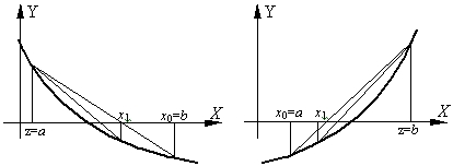
Newton's method is also intended to refine the root on the interval [ a, b], at the ends of which the function f(x) takes values of different signs. But this method uses additional information about the function f(x). As a result, it has faster convergence, but at the same time, it is applicable to a narrower class of functions, and its convergence is not always guaranteed.
When separating the roots of a function, it should be taken into account that the application of Newton's method requires that the function be monotonic and twice differentiable, with the second derivative f''(x) should not change sign on this interval.
The convergence of the iteration sequence obtained in Newton’s method depends on the choice of the initial approximation x 0. In general, if the interval [ a, b] containing the root, and it is known that the function f(x) is monotonic on this interval, then as an initial approximation x 0 you can select that boundary of the segment [ a, b], where the signs of the function coincide f(x) and second derivative f''(x). This choice of initial approximation guarantees the convergence of Newton's method, provided that the function is monotonic on the root localization segment.
Let us know the initial approximation to the root x 0. Let us draw a tangent to the curve at this point y= f(x) (Fig. 6). This tangent will intersect the x-axis at a point that we will consider as the next approximation.